Back to Article
Testing for differences between sites using three different sampling designs
Download Source

Testing for differences between sites using three different sampling designs

Author

Alex Koiter

Load Libraries

In [1]:
library(tidyverse)
── Attaching core tidyverse packages ──────────────────────── tidyverse 2.0.0 ──
✔ dplyr     1.1.4     ✔ readr     2.1.4
✔ forcats   1.0.0     ✔ stringr   1.5.1
✔ ggplot2   3.5.0     ✔ tibble    3.2.1
✔ lubridate 1.9.2     ✔ tidyr     1.3.1
✔ purrr     1.0.2     
── Conflicts ────────────────────────────────────────── tidyverse_conflicts() ──
✖ dplyr::filter() masks stats::filter()
✖ dplyr::lag()    masks stats::lag()
ℹ Use the conflicted package (<http://conflicted.r-lib.org/>) to force all conflicts to become errors
library(scales)

Attaching package: 'scales'

The following object is masked from 'package:purrr':

    discard

The following object is masked from 'package:readr':

    col_factor
library(viridis)
Loading required package: viridisLite

Attaching package: 'viridis'

The following object is masked from 'package:scales':

    viridis_pal
library(FSA)
## FSA v0.9.5. See citation('FSA') if used in publication.
## Run fishR() for related website and fishR('IFAR') for related book.
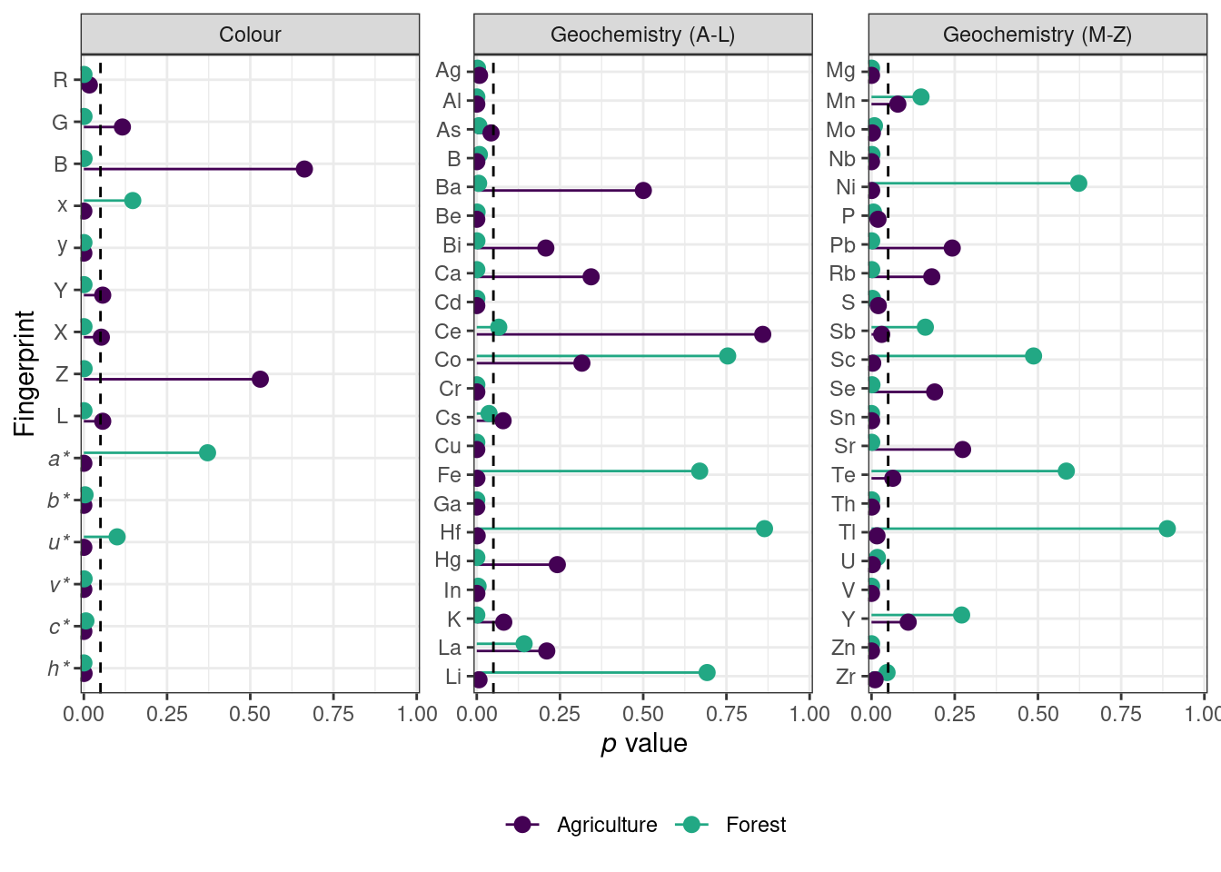
library(patchwork)

Load data

In [2]:
psa <- read.csv(here::here("./notebooks/PSA_data.csv")) %>%
  rename(site = Site) %>%
  select(site, sample_number, sampling_design, dx_50, specific_surface_area) %>%
  filter(sampling_design != "Fine scale")  

om <- read.csv(here::here("./notebooks/OM_data.csv")) %>%
  rename(site = Site, sampling_design = Sampling_Design, sample_number = Sample_Number) %>%
  select(OM, site, sampling_design, sample_number) %>%
  filter(sampling_design != "Fine scale") %>%
  mutate(site = recode(site, Agricultural = "Agriculture")) 

geo <- read.csv(here::here("./notebooks/Geochemistry analysis - Copy 2.csv")) %>%
  select(-X) %>%
  rename(sampling_design = sample_design) %>%
  filter(sampling_design != "Fine scale")  

colour <- read.csv(here::here("./notebooks/final results revised.csv")) %>%
  select(-X.1) %>%
  rename(sampling_design = sample_design) %>%
  filter(sampling_design != "Fine scale") 

Kruskal Wallis test

Colour

In [3]:
kruskal_colour <- colour %>%
  pivot_longer(cols = X:B, names_to = "Fingerprint", values_to = "value") %>%
  nest(data = c(-Fingerprint, - site)) %>%
  mutate(k_test = map(data, ~kruskal.test(value ~ sampling_design, data = .))) %>%
  mutate(p_value = map_dbl(k_test, ~ .$p.value)) %>%
  select(site, Fingerprint,p_value)%>%
  mutate(type = "colour")
  
kruskal_colour 
# A tibble: 30 × 4
   site        Fingerprint    p_value type  
   <chr>       <chr>            <dbl> <chr> 
 1 Agriculture X           0.0526     colour
 2 Agriculture Y           0.0567     colour
 3 Agriculture Z           0.530      colour
 4 Agriculture x           0.0000370  colour
 5 Agriculture y           0.00000552 colour
 6 Agriculture u           0.0000173  colour
 7 Agriculture v           0.00000769 colour
 8 Agriculture L           0.0567     colour
 9 Agriculture a           0.0000362  colour
10 Agriculture b           0.0000104  colour
# ℹ 20 more rows

Geochemistry

In [4]:
kruskal_geo <- geo %>%
  pivot_longer(cols = Ag:Zr, names_to = "Fingerprint", values_to = "value") %>%
  nest(data = c(-Fingerprint, - site)) %>%
  mutate(k_test = map(data, ~kruskal.test(value ~ sampling_design, data = .))) %>%
  mutate(p_value = map_dbl(k_test, ~ .$p.value)) %>%
  select(site, Fingerprint,p_value) %>%
  mutate(type = "geochemistry") %>%
  filter(Fingerprint %in% c("Ag", "Al", "As","B","Ba","Be","Bi","Ca","Cd","Ce","Co", "Cr", "Cs", "Cu", "Fe", "Ga", "Hf", "Hg", "In", "K", "La", "Li", "Mg", "Mn", "Mo", "Nb", "Ni", "P", "Pb", "Rb", "S", "Sb", "Sc", "Se", "Sn", "Sr", "Te", "Th", "Tl", "U", "V", "Y", "Zn", "Zr"))
kruskal_geo 
# A tibble: 88 × 4
   site   Fingerprint  p_value type        
   <chr>  <chr>          <dbl> <chr>       
 1 Forest Ag          0.00218  geochemistry
 2 Forest Al          0.000205 geochemistry
 3 Forest As          0.00640  geochemistry
 4 Forest B           0.00786  geochemistry
 5 Forest Ba          0.00558  geochemistry
 6 Forest Be          0.000968 geochemistry
 7 Forest Bi          0.000413 geochemistry
 8 Forest Ca          0.000155 geochemistry
 9 Forest Cd          0.000229 geochemistry
10 Forest Ce          0.0661   geochemistry
# ℹ 78 more rows

plotting

In [5]:
plot_ele <- c("Ag", "Al", "As", "B",  "Ba", "Be", "Bi", "Ca", "Cd", "Ce", "Co", "Cr", "Cs", "Cu", "Fe", "Ga", "Hf", "Hg", "In", "K",  "La", "Li")

kruskal_p <- kruskal_colour %>%
  bind_rows(kruskal_geo) %>%
  mutate(start = 0) %>%
  mutate(group = case_when(type == "colour" ~ "Colour",
                           type == "geochemistry" & Fingerprint %in% plot_ele ~ "Geochemistry (A-L)",
                           type == "geochemistry" & !Fingerprint %in% plot_ele ~ "Geochemistry (M-Z)")) %>%
  mutate(
    Fingerprint = fct_relevel(
      Fingerprint,
      c("R", "G", "B", "x", "y", "Y", "X", "Z", "L", "a", "b", "u", "v", "c", "h")),
    Fingerprint = fct_relevel(Fingerprint, c("Ag", "Al", "As"), 
                              after = which(levels(Fingerprint) == "B") - 1),
    Fingerprint = fct_relevel(Fingerprint, c("Mg", "Mn", "Mo", "Nb", "Ni", "P", "Pb", "Rb", "S", 
                                             "Sb", "Sc", "Se", "Sn", "Sr", "Te", "Th", "Tl", "U", "V"), 
                              after = which(levels(Fingerprint) == "Y") - 1)) %>%
  mutate(Fingerprint = fct_recode(
    Fingerprint, 
    "italic(`a*`)" = "a", "italic(`b*`)" = "b", "italic(`c*`)" = "c", "italic(`h*`)" = "h", 
    "italic(`u*`)" = "u",  "italic(`v*`)" = "v"))

p1 <- ggplot(data = kruskal_p, aes(y = fct_relevel(Fingerprint, rev), x = p_value, colour = site)) +
  #geom_point(position = position_dodge(width = 0.2)) +
  geom_pointrange(aes(xmax= p_value, xmin = 0), position = position_dodge(width = 0.5), linewidth = 0.5) +
  geom_vline(xintercept = 0.05, linetype = "dashed") +
  theme_bw() +
  scale_x_continuous(expand = c(0.01,0), limits = c(0,1)) +
  scale_y_discrete(labels = label_parse()) +
  scale_colour_viridis_d(begin = 0, end = 0.6) +
  theme(legend.position = "bottom",
        legend.title = element_blank()) +
  labs(x = expression(paste(italic("p"), " value")), y = "Fingerprint") +
  facet_wrap(~group, scales = "free_y")

p1

Dunns test

Post-hoc test

In [6]:
kw_geo_pass <- filter(kruskal_geo, p_value <0.05) %>%
  rename("fingerprint" = "Fingerprint")

dunngeo <- geo %>%
  pivot_longer(cols = Ag:Zr, names_to = "fingerprint", values_to = "value") %>%
  semi_join(kw_geo_pass, by = c("fingerprint", "site")) %>%
  select(-sample_number) %>%
  mutate(sampling_design = as.factor(sampling_design)) %>%
  nest(data = c(-fingerprint, - site)) %>%
  mutate(dunn_test = map(data, ~dunnTest(value ~ sampling_design, data = .,
                                         method = "bh"))) %>%
  mutate(p_value = map(dunn_test, ~ .$res)) %>%
  unnest(p_value) %>%
  mutate(type = "Geochemistry")

kw_colour_pass <- filter(kruskal_colour, p_value <0.05) %>%
  rename("fingerprint" = "Fingerprint")

dunncolour <- colour %>%
  pivot_longer(cols = X:B, names_to = "fingerprint", values_to = "value") %>%
  semi_join(kw_colour_pass, by = c("fingerprint", "site")) %>%
  select(-sample_number) %>%
  mutate(sampling_design = as.factor(sampling_design)) %>%
  nest(data = c(-fingerprint, - site)) %>%
  mutate(dunn_test = map(data, ~dunnTest(value ~ sampling_design, data = .,
                                         method = "bh"))) %>%
  mutate(p_value = map(dunn_test, ~ .$res)) %>%
  unnest(p_value) %>%
  mutate(type = "Colour")

Plotting

In [7]:
dunn_p <- dunncolour %>%
  bind_rows(dunngeo) %>%
  mutate(start = 0) %>%
  mutate(group = case_when(type == "Colour" ~ "Colour",
                           type == "Geochemistry" & fingerprint %in% plot_ele ~ "Geochemistry (A-L)",
                           type == "Geochemistry" & !fingerprint %in% plot_ele ~ "Geochemistry (M-Z)")) %>%
  mutate(
    fingerprint = fct_relevel(
      fingerprint,
      c("R", "G", "B", "x", "y", "Y", "X", "Z", "L", "a", "b", "u", "v", "c", "h")),
    fingerprint = fct_relevel(fingerprint, c("Ag", "Al", "As"), 
                              after = which(levels(fingerprint) == "B") - 1),
    fingerprint = fct_relevel(fingerprint, c("Mg", "Mo", "Nb", "Ni", "P", "Pb", "Rb", "S", 
                                             "Sb", "Sc", "Se", "Sn", "Sr", "Th", "Tl", "U", "V"), 
                              after = which(levels(fingerprint) == "Y") - 1)) %>%
  mutate(fingerprint = fct_recode(
    fingerprint, 
    "italic(`a*`)" = "a", "italic(`b*`)" = "b", "italic(`c*`)" = "c", "italic(`h*`)" = "h", 
    "italic(`u*`)" = "u",  "italic(`v*`)" = "v"))


p2 <- ggplot(data = dunn_p, aes(y = fct_relevel(fingerprint, rev), x = P.adj, fill = Comparison)) +
  #geom_point(position = position_dodge(width = 0.2)) +
  geom_pointrange(aes(xmax= P.adj, xmin = 0), position = position_dodge(width = 0.5), linewidth = 0.2, shape = 21, stroke = 0.5) +
  geom_vline(xintercept = 0.05, linetype = "dashed") +
  theme_bw() +
  scale_x_continuous(expand = c(0.01,0), limits = c(0,1)) +
  scale_y_discrete(labels = label_parse()) +
  scale_fill_viridis_d(begin = 0, end = 0.9, alpha = 0.8) +
  theme(legend.position = "bottom",
        legend.title = element_blank()) +
  labs(x = expression(paste("Adjusted ", italic("p"), " value")), y = "Fingerprint") +
  facet_grid(group ~ site,scales = "free")
p2

p3 <- ggplot(data = filter(dunn_p, type == "Colour"), aes(y = fct_relevel(fingerprint, rev), x = P.adj, fill = Comparison)) +
  #geom_point(position = position_dodge(width = 0.2)) +
  geom_pointrange(aes(xmax= P.adj, xmin = 0), position = position_dodge(width = 0.5), linewidth = 0.2, shape = 21, stroke = 0.5) +
  geom_vline(xintercept = 0.05, linetype = "dashed") +
  theme_bw() +
  scale_x_continuous(expand = c(0.01,0), limits = c(0,1)) +
  scale_y_discrete(labels = label_parse()) +
  scale_fill_viridis_d(begin = 0, end = 0.9, alpha = 0.8) +
  theme(axis.text.x = element_text(angle = 45, vjust = 1, hjust = 1),
        legend.title = element_blank()) +
  labs(x = expression(paste("Adjusted ", italic("p"), " value")), y = "Fingerprint") +
  facet_wrap(~ site,scales = "free")
p3

p4 <- ggplot(data = filter(dunn_p, type == "Geochemistry", group == "Geochemistry (A-L)"), aes(y = fct_relevel(fingerprint, rev), x = P.adj, fill = Comparison)) +
  #geom_point(position = position_dodge(width = 0.2)) +
  geom_pointrange(aes(xmax= P.adj, xmin = 0), position = position_dodge(width = 0.5), linewidth = 0.2, shape = 21, stroke = 0.5) +
  geom_vline(xintercept = 0.05, linetype = "dashed") +
  theme_bw() +
  scale_x_continuous(expand = c(0.01,0), limits = c(0,1)) +
  scale_y_discrete(labels = label_parse()) +
  scale_fill_viridis_d(begin = 0, end = 0.9, alpha = 0.8) +
  theme(axis.text.x = element_text(angle = 45, vjust = 1, hjust = 1),
        axis.title.x = element_blank(),
        legend.title = element_blank()) +
  labs(x = expression(paste("Adjusted ", italic("p"), " value")), y = "Fingerprint") +
  facet_wrap(~ site,scales = "free")
p4

p5 <- ggplot(data = filter(dunn_p, type == "Geochemistry", group != "Geochemistry (A-L)"), aes(y = fct_relevel(fingerprint, rev), x = P.adj, fill = Comparison)) +
  #geom_point(position = position_dodge(width = 0.2)) +
  geom_pointrange(aes(xmax= P.adj, xmin = 0), position = position_dodge(width = 0.5), linewidth = 0.2, shape = 21, stroke = 0.5) +
  geom_vline(xintercept = 0.05, linetype = "dashed") +
  theme_bw() +
  scale_x_continuous(expand = c(0.01,0), limits = c(0,1)) +
  scale_y_discrete(labels = label_parse()) +
  scale_fill_viridis_d(begin = 0, end = 0.9, alpha = 0.8) +
  theme(axis.text.x = element_text(angle = 45, vjust = 1, hjust = 1),
        axis.title.y = element_blank(),
        axis.title.x = element_blank(),
        legend.title = element_blank()) +
  labs(x = expression(paste("Adjusted ", italic("p"), " value")), y = "Fingerprint") +
  facet_wrap(~ site,scales = "free")
p5

In [8]:
p6 <- p4 + p5 + p3 + guide_area() + 
  plot_layout(guides = 'collect') + plot_layout(axis_titles = "collect")
p6
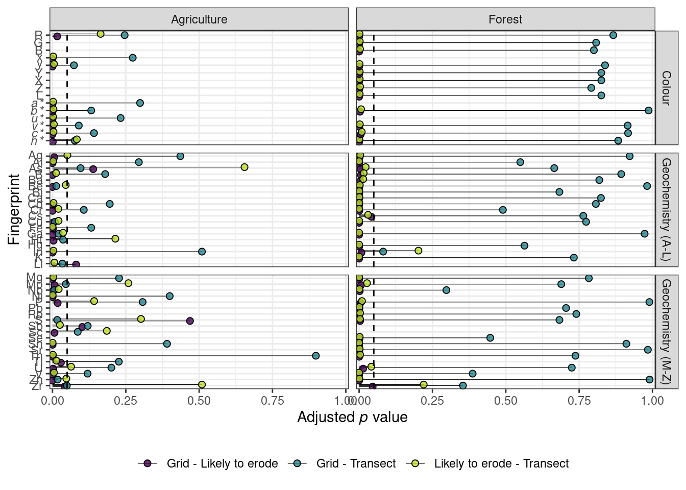
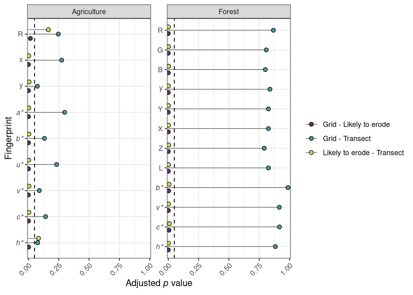
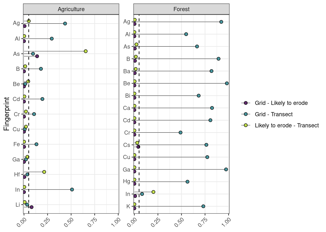
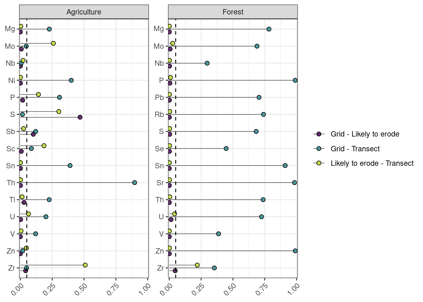
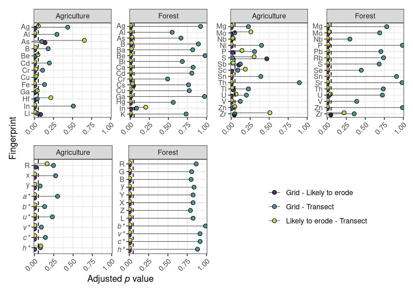
Results for the pair-wise Dunn’s post-hoc test to determine differences in fingerprint properties between the three sampling designs for each site. Dashed line represents an α value of 0.05. Fingerprints that showed no significant differences (p value > 0.05) following the Kruskal Wallis test are not included.