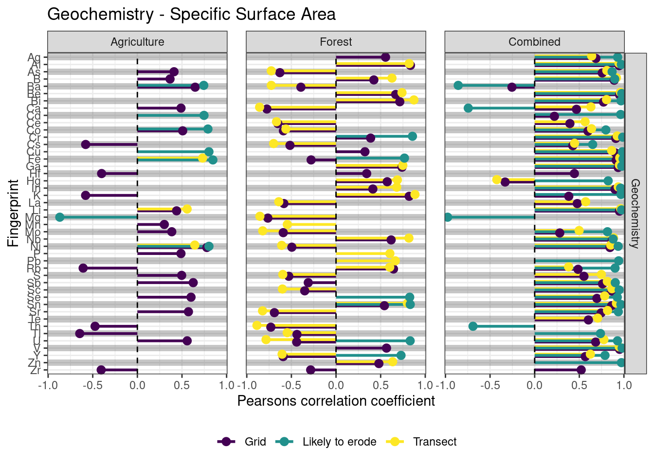
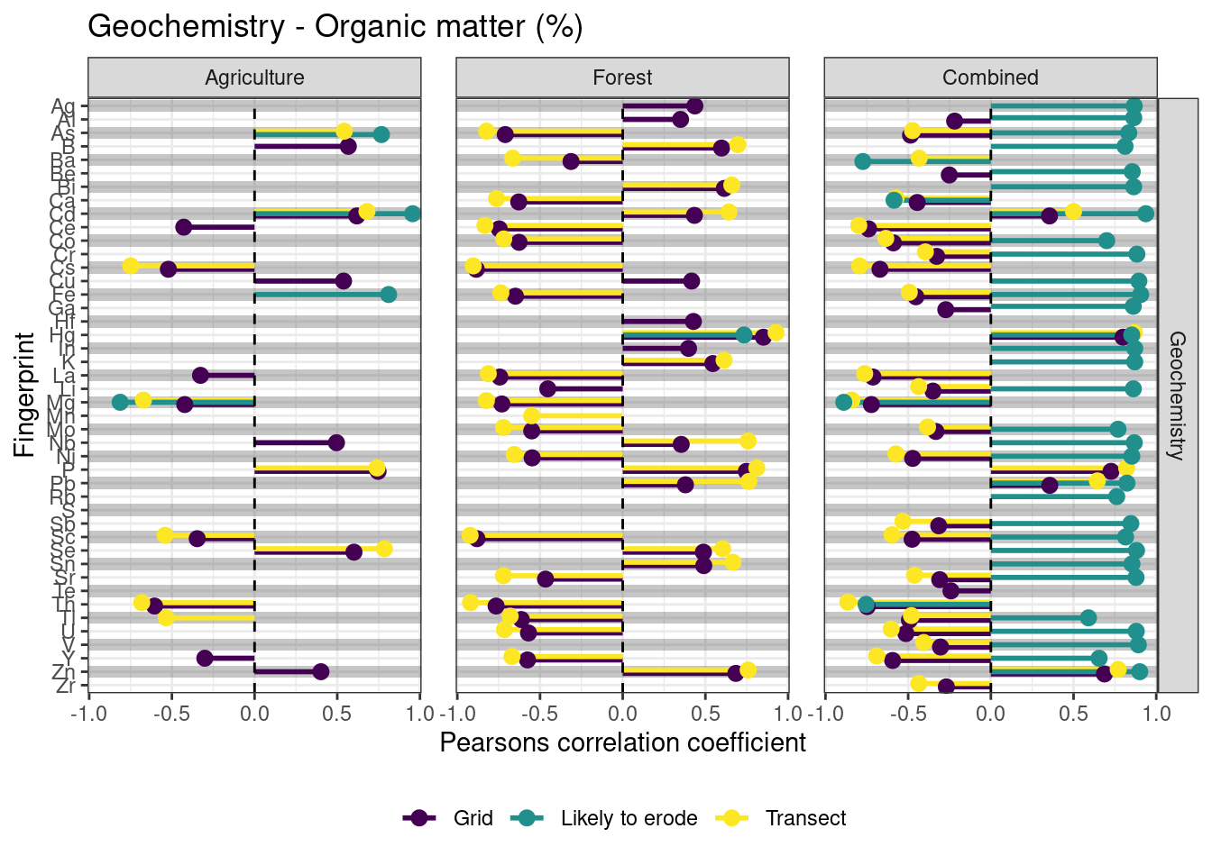
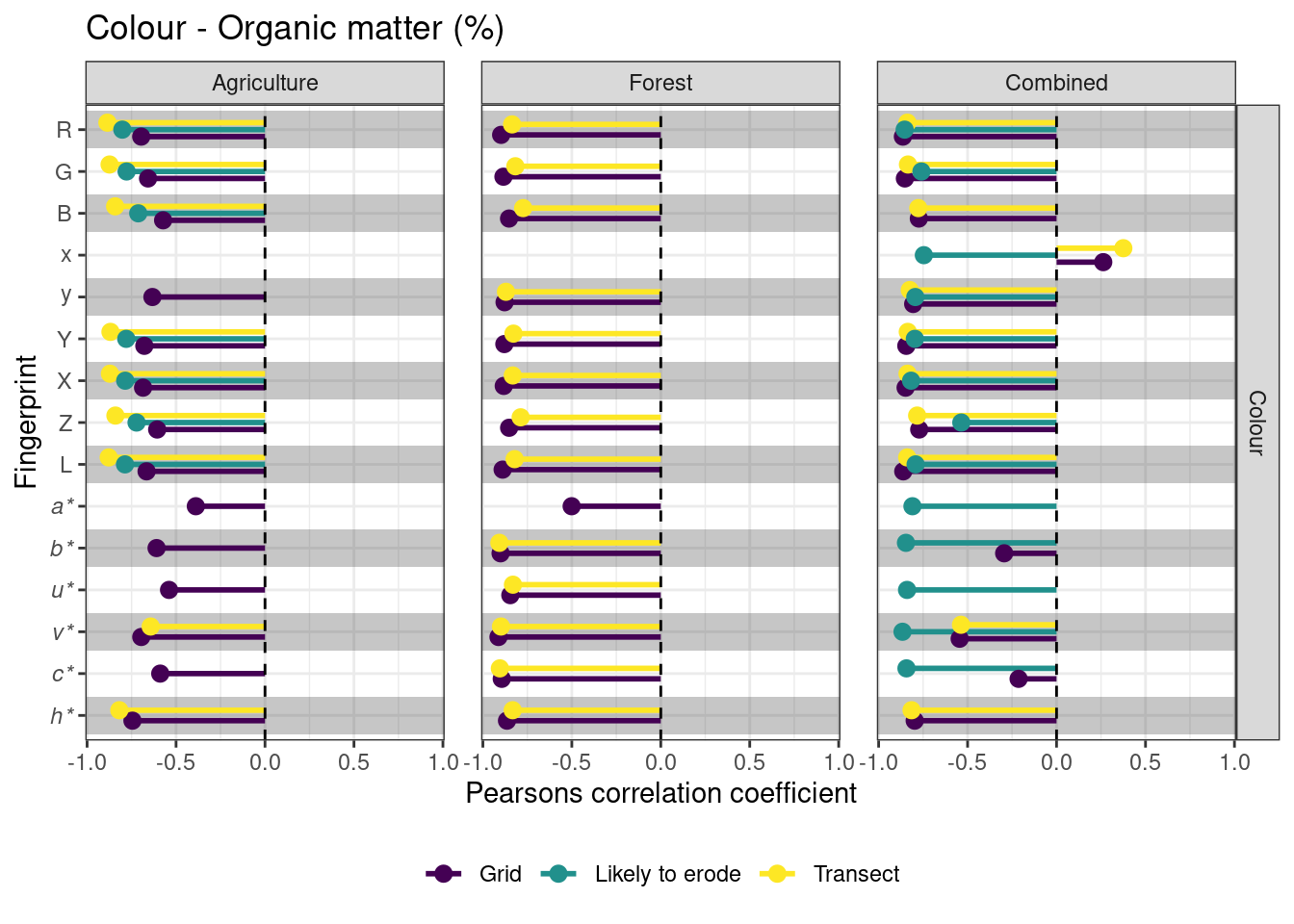
Correlations between soil colour and geochemical properties and SSA and SOM
Author
Alex Koiter
Load Libraries
In [1]:
library(tidyverse)
── Attaching core tidyverse packages ──────────────────────── tidyverse 2.0.0 ──
✔ dplyr     1.1.4     ✔ readr     2.1.4
✔ forcats   1.0.0     ✔ stringr   1.5.1
✔ ggplot2   3.5.0     ✔ tibble    3.2.1
✔ lubridate 1.9.2     ✔ tidyr     1.3.1
✔ purrr     1.0.2
── Conflicts ────────────────────────────────────────── tidyverse_conflicts() ──
✖ dplyr::filter() masks stats::filter()
✖ dplyr::lag()    masks stats::lag()
ℹ Use the conflicted package (<http://conflicted.r-lib.org/>) to force all conflicts to become errors
library(patchwork)library(scales)
Attaching package: 'scales'

The following object is masked from 'package:purrr':

    discard

The following object is masked from 'package:readr':

    col_factor
library(viridis)
Loading required package: viridisLite

Attaching package: 'viridis'

The following object is masked from 'package:scales':

    viridis_pal
Joining with `by = join_by(sample_number, site, sampling_design)`
Joining with `by = join_by(sample_number, site, sampling_design)`
Warning: There were 2 warnings in `mutate()`.
The first warning was:
ℹ In argument: `ssa_test = map(data, ~cor.test(.$value,
  .$specific_surface_area, method = "pearson"))`.
Caused by warning in `cor()`:
! the standard deviation is zero
ℹ Run `dplyr::last_dplyr_warnings()` to see the 1 remaining warning.
Warning: There were 2 warnings in `mutate()`.
The first warning was:
ℹ In argument: `d50_test = map(data, ~cor.test(.$value,
  .$specific_surface_area, method = "pearson"))`.
Caused by warning in `cor()`:
! the standard deviation is zero
ℹ Run `dplyr::last_dplyr_warnings()` to see the 1 remaining warning.
Warning: There were 2 warnings in `mutate()`.
The first warning was:
ℹ In argument: `om_test = map(data, ~cor.test(.$value, .$OM, method =
  "pearson"))`.
Caused by warning in `cor()`:
! the standard deviation is zero
ℹ Run `dplyr::last_dplyr_warnings()` to see the 1 remaining warning.
corr_geo
# A tibble: 264 × 10
   site   sampling_design Fingerprint p_value_ssa estimate_ssa p_value_d50
   <chr>  <chr>           <chr>             <dbl>        <dbl>       <dbl>
 1 Forest Grid            Ag             2.89e- 5        0.555    2.89e- 5
 2 Forest Grid            Al             5.39e-14        0.834    5.39e-14
 3 Forest Grid            As             9.84e- 7       -0.629    9.84e- 7
 4 Forest Grid            B              2.15e- 3        0.424    2.15e- 3
 5 Forest Grid            Ba             4.69e- 3       -0.394    4.69e- 3
 6 Forest Grid            Be             1.11e- 7        0.669    1.11e- 7
 7 Forest Grid            Bi             5.61e- 9        0.715    5.61e- 9
 8 Forest Grid            Ca             3.95e-11       -0.775    3.95e-11
 9 Forest Grid            Cd             2.20e- 1        0.177    2.20e- 1
10 Forest Grid            Ce             2.95e- 7       -0.652    2.95e- 7
# ℹ 254 more rows
# ℹ 4 more variables: estimate_d50 <dbl>, p_value_om <dbl>, estimate_om <dbl>,
#   type <chr>
`geom_smooth()` using formula = 'y ~ x'
`geom_smooth()` using formula = 'y ~ x'
`geom_smooth()` using formula = 'y ~ x'
`geom_smooth()` using formula = 'y ~ x'
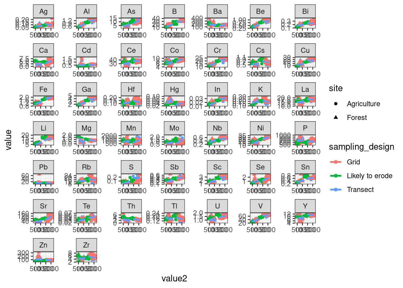
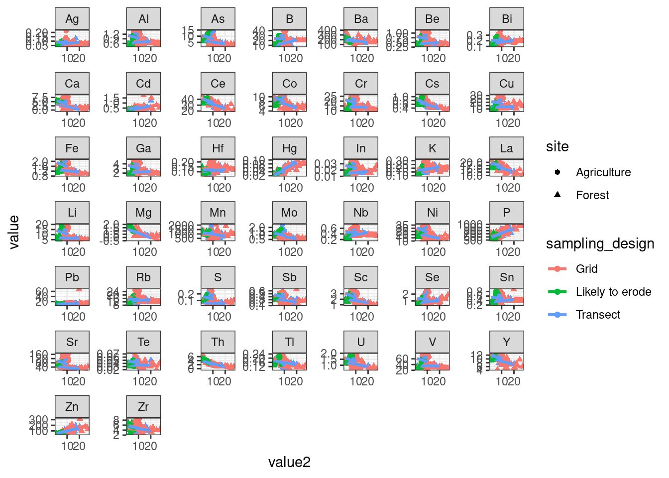
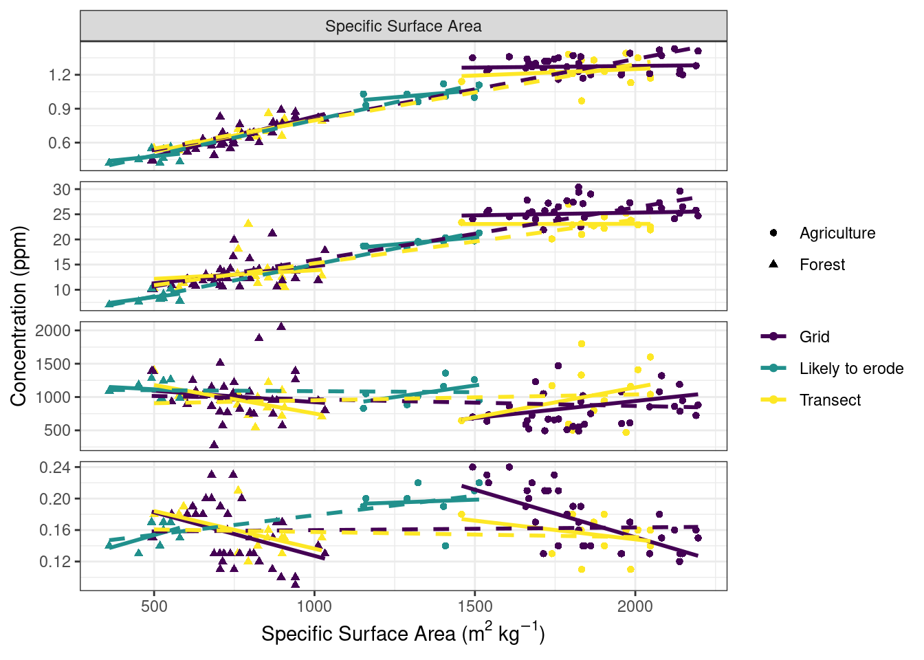
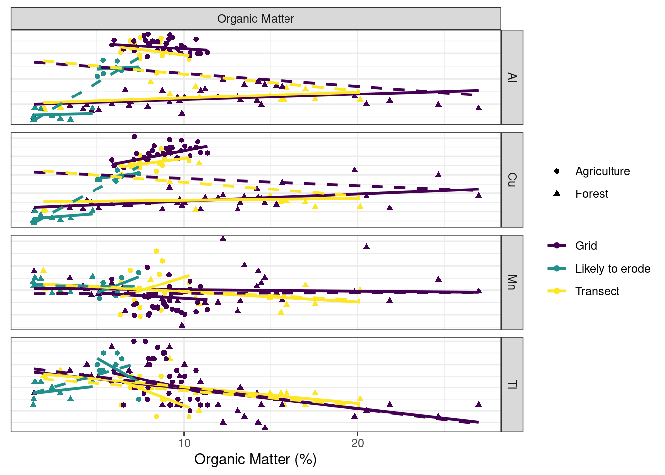
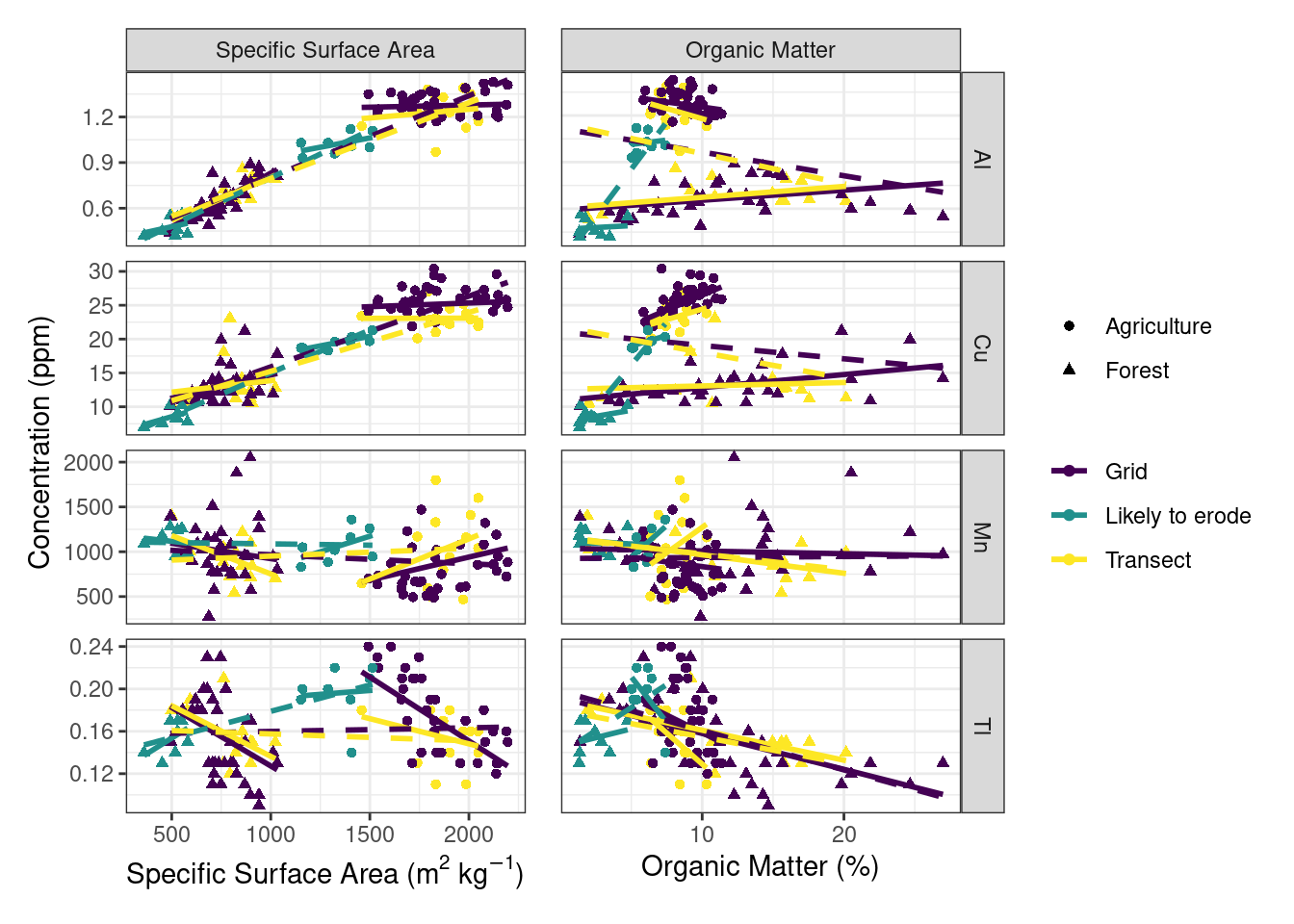
Exploring the relation between select geochemical concentrations and specific surface area and soil organic matter content. Solid lines indicate linear relation for each site and sampling design independently and dashed lines indicate linear relation for each sampling design with data combined across both sites.
`geom_smooth()` using formula = 'y ~ x'
`geom_smooth()` using formula = 'y ~ x'
`geom_smooth()` using formula = 'y ~ x'
`geom_smooth()` using formula = 'y ~ x'
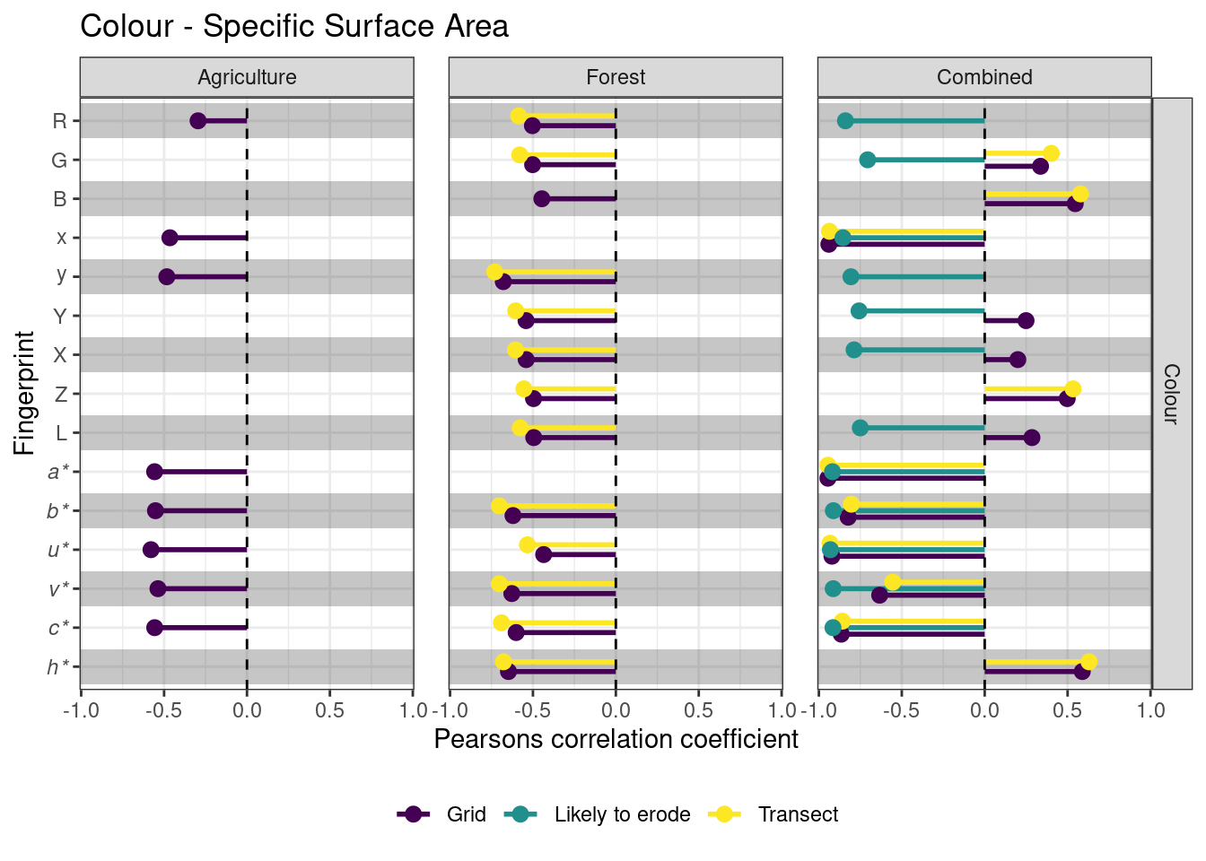
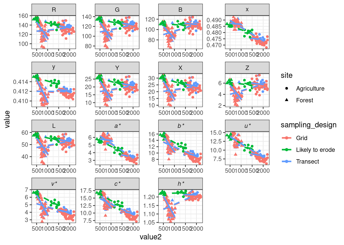
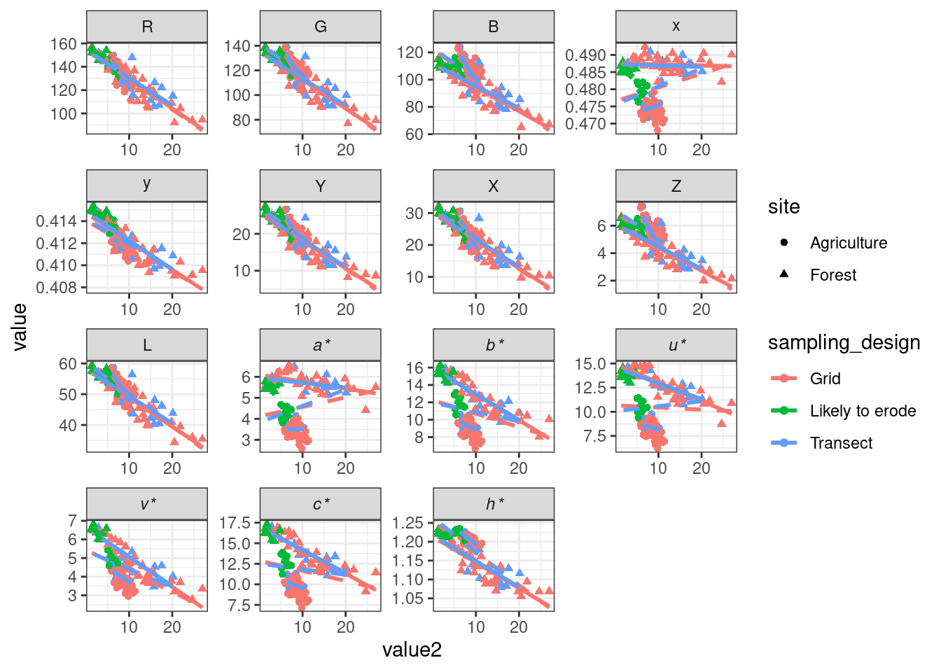
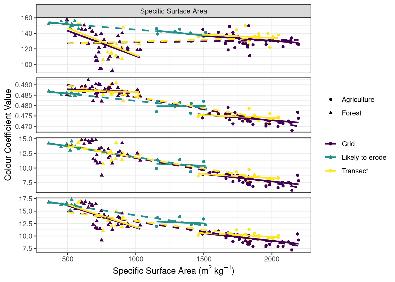
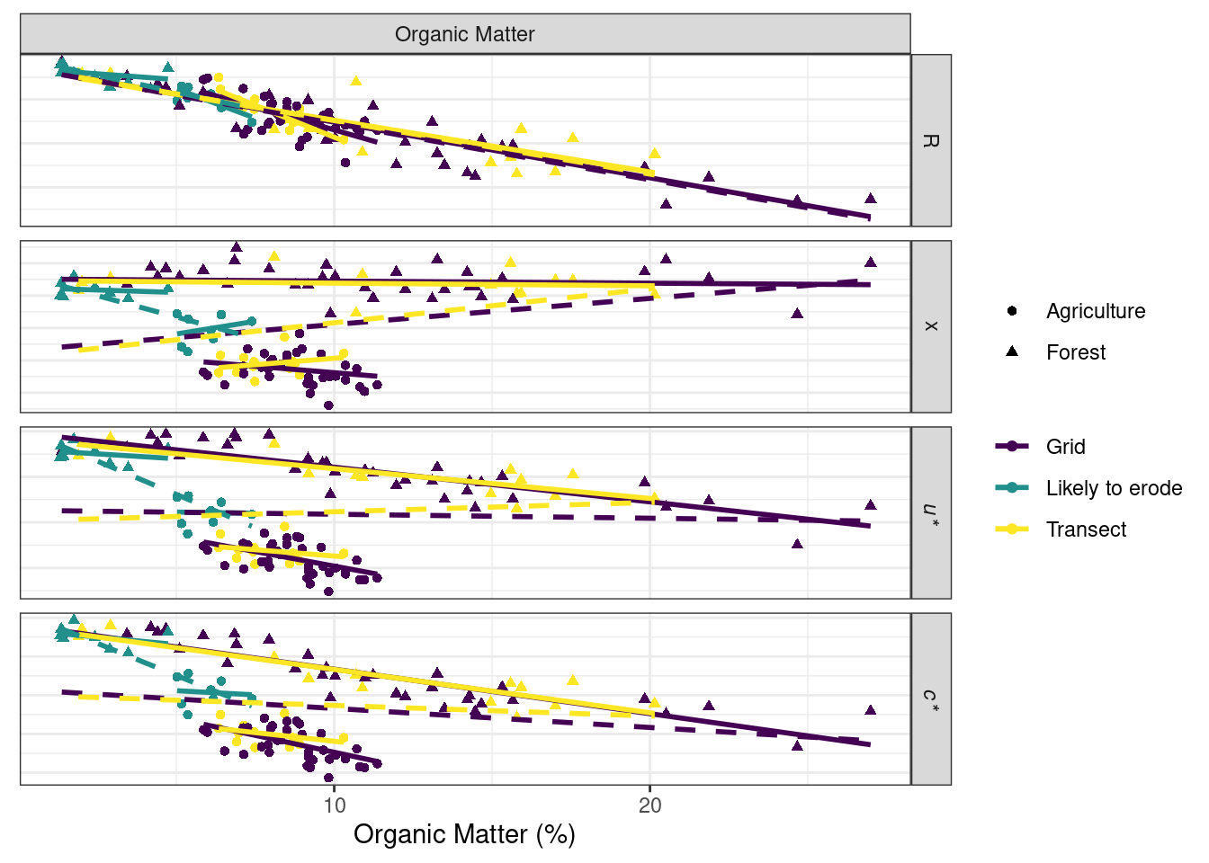
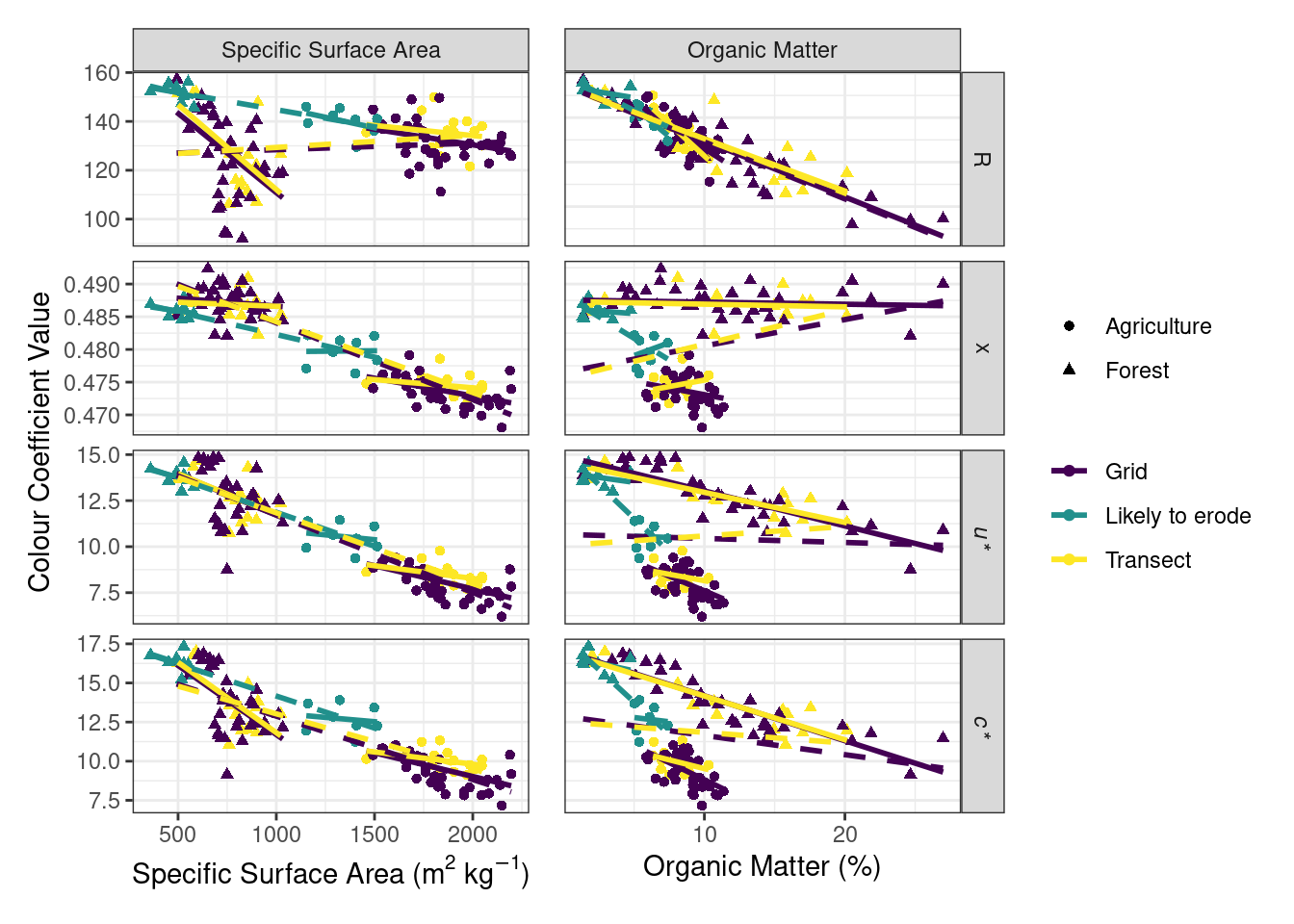
Exploring the relation between select colour coefficients and specific surface area and soil organic matter content. Solid lines indicate linear relation for each site and sampling design independently and dashed lines indicate linear relation for each sampling design with data combined across both sites.