Rows: 63000 Columns: 10
── Column specification ────────────────────────────────────────────────────────
Delimiter: ","
chr (2): model_filename, run
dbl (4): prop_forest, alpha.prior, Agriculture, Forest
lgl (4): mix, source, discr, model

ℹ Use `spec()` to retrieve the full column specification for this data.
ℹ Specify the column types or set `show_col_types = FALSE` to quiet this message.
likely <-read_csv(here::here("./notebooks/Mixtures_likely/likely_final_results.csv")) %>%mutate(sampling_design ="Likely to erode")
Rows: 63000 Columns: 10
── Column specification ────────────────────────────────────────────────────────
Delimiter: ","
chr (2): model_filename, run
dbl (4): prop_forest, alpha.prior, Agriculture, Forest
lgl (4): mix, source, discr, model

ℹ Use `spec()` to retrieve the full column specification for this data.
ℹ Specify the column types or set `show_col_types = FALSE` to quiet this message.
all <- grid %>%bind_rows(transect, likely) %>%mutate(sampling_design =fct_relevel(sampling_design, "Grid", "Transect", "Likely to erode"))
Plotting
In [3]:
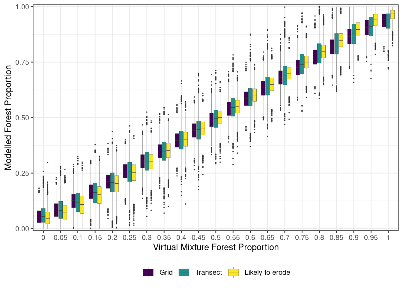
supfig6 <-ggplot(data = all, aes(x =as.factor(prop_forest), y = Forest, fill = sampling_design)) +geom_boxplot(size =0.1, outlier.size =0.1) +theme_bw() +scale_y_continuous(expand =c(0,0.01)) +labs(y ="Modelled Forest Proportion", x ="Virtual Mixture Forest Proportion") +theme(legend.position ="bottom", legend.title =element_blank()) +scale_fill_viridis_d()supfig6
`summarise()` has grouped output by 'sampling_design', 'prop_forest'. You can
override using the `.groups` argument.
`summarise()` has grouped output by 'sampling_design'. You can override using
the `.groups` argument.
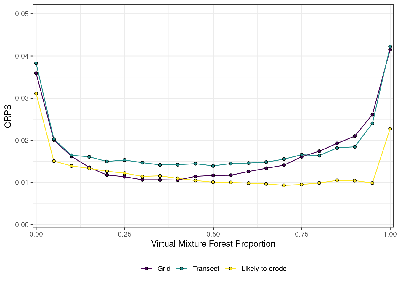
summary_2 <- all %>%mutate(prop_ag =1- prop_forest) %>%group_by(prop_forest, sampling_design) %>%summarise(CRPS_forest =crps_sample(y =unique(prop_forest), dat = Forest),CRPS_ag =crps_sample(y =unique(prop_ag), dat = Agriculture)) %>%group_by(sampling_design) %>%summarise(Forest =mean(CRPS_forest),Agriculture =mean(CRPS_ag)) %>%pivot_longer(cols =c(Forest, Agriculture), names_to ="source", values_to ="CRPS")
`summarise()` has grouped output by 'prop_forest'. You can override using the
`.groups` argument.
CRPS_plot <- all %>%mutate(prop_ag =1- prop_forest) %>%group_by(prop_forest, prop_ag, sampling_design) %>%summarise(Forest =crps_sample(y =unique(prop_forest), dat = Forest),Agriculture =crps_sample(y =unique(prop_ag), dat = Agriculture))
`summarise()` has grouped output by 'prop_forest', 'prop_ag'. You can override
using the `.groups` argument.