Rows: 63000 Columns: 10
── Column specification ────────────────────────────────────────────────────────
Delimiter: ","
chr (2): model_filename, run
dbl (4): prop_forest, alpha.prior, Agriculture, Forest
lgl (4): mix, source, discr, model

ℹ Use `spec()` to retrieve the full column specification for this data.
ℹ Specify the column types or set `show_col_types = FALSE` to quiet this message.
all_likely <-read_csv(here::here("./notebooks/Mixtures_all_likely/likely_final_results.csv")) %>%mutate(sampling_design ="Likely to erode")
Rows: 63000 Columns: 10
── Column specification ────────────────────────────────────────────────────────
Delimiter: ","
chr (2): model_filename, run
dbl (4): prop_forest, alpha.prior, Agriculture, Forest
lgl (4): mix, source, discr, model

ℹ Use `spec()` to retrieve the full column specification for this data.
ℹ Specify the column types or set `show_col_types = FALSE` to quiet this message.
all <- all_grid %>%bind_rows(all_transect, all_likely) %>%mutate(sampling_design =fct_relevel(sampling_design, "Grid", "Transect", "Likely to erode"))
Plotting
In [3]:
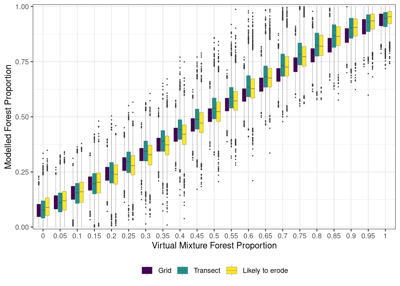
mixing_plot1 <-ggplot(data = all, aes(x =as.factor(prop_forest), y = Forest, fill = sampling_design)) +geom_boxplot(size =0.1, outlier.size =0.1) +theme_bw() +scale_y_continuous(expand =c(0,0.01)) +labs(y ="Modelled Forest Proportion", x ="Virtual Mixture Forest Proportion") +theme(legend.position ="bottom", legend.title =element_blank()) +scale_fill_viridis_d()mixing_plot1
Comparison of the posterior distribution of the modeled proportion of forest source to the proportion of forest source in the virtual mixtures for each of the three sampling designs.
In [4]:
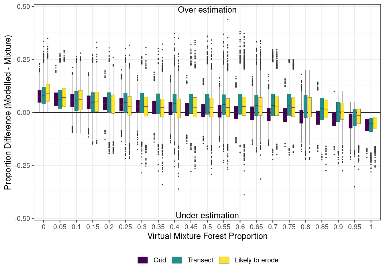
mixing_plot2 <-ggplot(data = all, aes(x =as.factor(prop_forest), y = Forest - prop_forest, fill = sampling_design)) +geom_hline(yintercept =0) +geom_boxplot(size =0.1, outlier.size =0.1) +theme_bw() +scale_y_continuous(expand =c(0,0.01), limits =c(-0.5, 0.5)) +labs(y ="Proportion Difference (Modelled - Mixture)", x ="Virtual Mixture Forest Proportion") +theme(legend.position ="bottom", legend.title =element_blank()) +scale_fill_viridis_d() +annotate(geom ="text", x ="0.5", y =0.5, label ="Over estimation", vjust =1) +annotate(geom ="text", x ="0.5", y =-0.5, label ="Under estimation", vjust =0)mixing_plot2
Differences in the proportions between modeled and virtual mixtures.
`summarise()` has grouped output by 'sampling_design', 'prop_forest'. You can
override using the `.groups` argument.
`summarise()` has grouped output by 'sampling_design'. You can override using
the `.groups` argument.
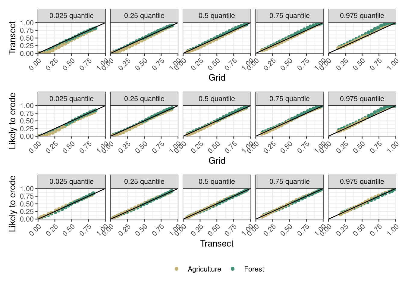
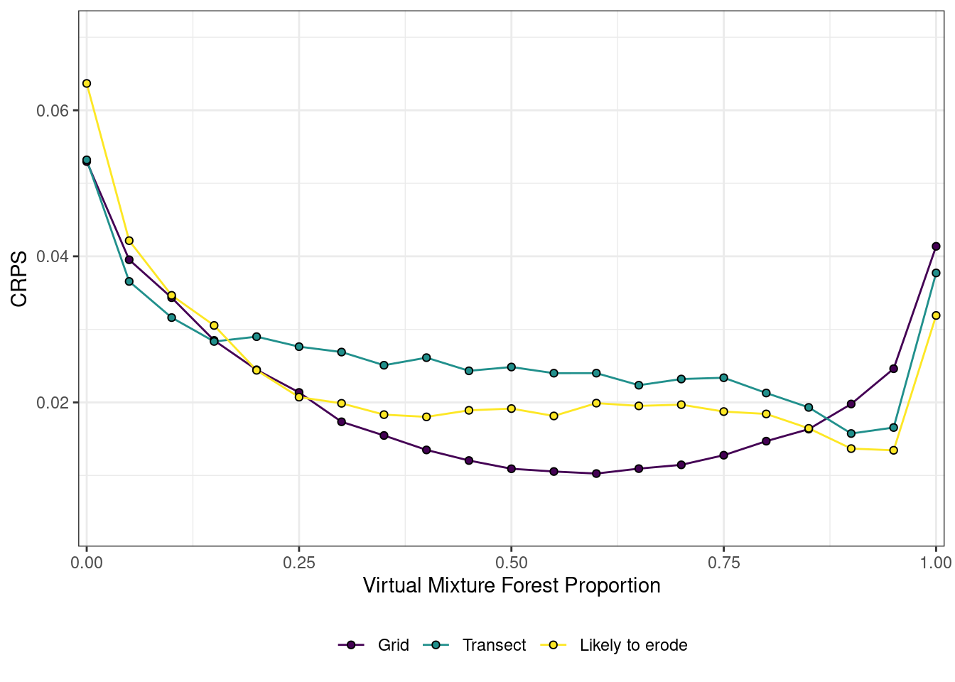
summary_2 <- all %>%mutate(prop_ag =1- prop_forest) %>%group_by(prop_forest, sampling_design) %>%summarise(CRPS_forest =crps_sample(y =unique(prop_forest), dat = Forest),CRPS_ag =crps_sample(y =unique(prop_ag), dat = Agriculture)) %>%group_by(sampling_design) %>%summarise(Forest =mean(CRPS_forest),Agriculture =mean(CRPS_ag)) %>%pivot_longer(cols =c(Forest, Agriculture), names_to ="source", values_to ="CRPS")
`summarise()` has grouped output by 'prop_forest'. You can override using the
`.groups` argument.
CRPS_plot <- all %>%mutate(prop_ag =1- prop_forest) %>%group_by(prop_forest, prop_ag, sampling_design) %>%summarise(Forest =crps_sample(y =unique(prop_forest), dat = Forest),Agriculture =crps_sample(y =unique(prop_ag), dat = Agriculture))
`summarise()` has grouped output by 'prop_forest', 'prop_ag'. You can override
using the `.groups` argument.