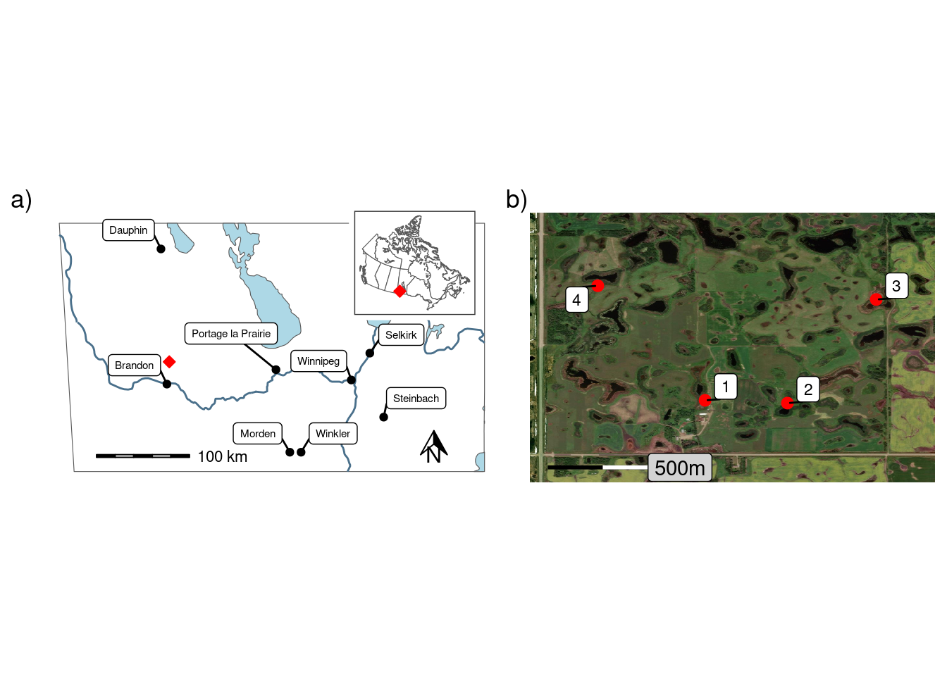
Back to Article
Map of study area
Download Source

Map of study area

Author

Alex Koiter

Load Libraries

In [1]:
library(tidyverse)
── Attaching core tidyverse packages ──────────────────────── tidyverse 2.0.0 ──
✔ dplyr     1.1.4     ✔ readr     2.1.5
✔ forcats   1.0.0     ✔ stringr   1.5.1
✔ ggplot2   3.5.1     ✔ tibble    3.2.1
✔ lubridate 1.9.3     ✔ tidyr     1.3.1
✔ purrr     1.0.2     
── Conflicts ────────────────────────────────────────── tidyverse_conflicts() ──
✖ dplyr::filter() masks stats::filter()
✖ dplyr::lag()    masks stats::lag()
ℹ Use the conflicted package (<http://conflicted.r-lib.org/>) to force all conflicts to become errors
library(ggspatial)
library(sf)
Linking to GEOS 3.10.2, GDAL 3.4.3, PROJ 8.2.1; sf_use_s2() is TRUE
library(rnaturalearth)
library(patchwork)
library(OpenStreetMap)

Important coordinants

Regional site location

In [2]:
site <- st_sfc(st_point(c(-99.924176, 50.056015)), crs = 4326)
box = c(xmin = -99.99, xmax = -99.924176 + 0.12, ymax = 50.056015 +.065, ymin = 50.056015 - 0.065)

Study plot locations

In [3]:
# sites <- st_as_sf(data.frame(site = c(1,2,3,4), lat = c(50.052525, 50.052209, 50.059208, 50.060235), long = c(-99.924242, -99.918429, -99.912849, -99.931591)), coords = c("long", "lat"), crs = 4362)
                                                                                              
sites <- data.frame(site = c(1,2,3,4), lat = c(50.052525, 50.052209, 50.059208, 50.060235), long = c(-99.924242, -99.918429, -99.912849, -99.931591))

Land use data of region

Get data

In [4]:
minnedosa_data <- "lcv_minnedosa_2004_2006_shp"
if (file.exists(minnedosa_data)) {
  print("The data already exists!")
} else {
  download.file("https://mli.gov.mb.ca/landuse/shp_zip_files/lcv_minnedosa_2004_2006_shp.zip", 
                destfile = "lcv_minnedosa_2004_2006_shp.zip")
  unzip("lcv_minnedosa_2004_2006_shp.zip", exdir = "lcv_minnedosa_2004_2006_shp")
}
[1] "The data already exists!"
brandon_data <- "lcv_brandon_2006_shp"
if (file.exists(brandon_data)) {
  print("The data already exists!")
} else {
  download.file("https://mli.gov.mb.ca/landuse/shp_zip_files/lcv_brandon_2006_shp.zip", 
                destfile = "lcv_brandon_2006_shp.zip")
  unzip("lcv_brandon_2006_shp.zip", exdir = "lcv_brandon_2006_shp")
}
[1] "The data already exists!"
In [5]:
sf_use_s2(FALSE)
Spherical geometry (s2) switched off
land <- st_read(here::here("./notebooks/lcv_brandon_2006_shp/lcv_brandon_2006.shp")) %>%
  bind_rows(st_read(here::here("./notebooks/lcv_minnedosa_2004_2006_shp/lcv_minnedosa_2004_2006.shp"))) %>%
  st_transform(crs = 4326) %>%
  st_crop(st_bbox(box, crs = 4326)) %>%
  mutate(Land_use = recode(CLASSNAME, "Agricultural Field" = "Agriculture", "Agri - Forage Field" = "Forage", "Water Body" = "Water", "Wetland - Treed Bog" = "Wetland", "Wetland - Marsh" = "Wetland", "Decidious Forest" = "Forest", "Open Decidious Forest" = "Forest", "Mixedwood Forest" = "Forest", "Forest Cut Blocks" = "Forest", "Coniferous Forest" = "Forest","Roads Trails Rail Lines" = "Other", "Sand and Gravel" = "Other", "Cultural Features" = "Other", "Range and Grassland" = "Forage", "Water Bodies" = "Water")) %>%
  # group_by(Land_use) %>%
  # summarise(do_union = TRUE) %>%
  mutate(Land_use = factor(Land_use, levels=c("Agriculture", "Forage", "Forest",  "Water", "Wetland", "Other")))
Reading layer `lcv_brandon_2006' from data source 
  `/home/alex/Dropbox/MBFI/MBFI riparian study/riparian-grazing-manuscript/notebooks/lcv_brandon_2006_shp/lcv_brandon_2006.shp' 
  using driver `ESRI Shapefile'
Simple feature collection with 145146 features and 5 fields
Geometry type: POLYGON
Dimension:     XY
Bounding box:  xmin: 429971 ymin: 5427260 xmax: 510011 ymax: 5542070
Projected CRS: UTM
Reading layer `lcv_minnedosa_2004_2006' from data source 
  `/home/alex/Dropbox/MBFI/MBFI riparian study/riparian-grazing-manuscript/notebooks/lcv_minnedosa_2004_2006_shp/lcv_minnedosa_2004_2006.shp' 
  using driver `ESRI Shapefile'
Simple feature collection with 160653 features and 5 fields
Geometry type: POLYGON
Dimension:     XY
Bounding box:  xmin: 429972 ymin: 5542070 xmax: 549972 ymax: 5656880
Projected CRS: UTM
although coordinates are longitude/latitude, st_intersection assumes that they
are planar
Warning: attribute variables are assumed to be spatially constant throughout
all geometries

Canada

In [6]:
canada <- ne_states(country = "Canada", returnclass = "sf") %>%
  st_transform(crs = 3348) 

Maps

Land use

In [7]:
p3 <- ggplot() +
  theme_bw() +
  geom_sf(data = land, aes(fill = Land_use), lwd = 0) +
  scale_fill_manual(values=c("#458B00",  "#CDAD00", "#006400","#009ACD", "#0096D194",  "#C1CDCD"), name = "Land use") +
  geom_point(data = sites, aes(x = long, y = lat), shape = 23, colour = "red", fill = "red", size = 2) +
  coord_sf(ylim = c(49.992, 50.1), xlim = c(-99.965, -99.80418), crs = 4326) +
  scale_y_continuous(expand = c(0,0)) +
  scale_x_continuous(expand = c(0,0)) +
  labs(tag = "b)") +
  annotation_scale(location = "bl",
                   height = unit(0.05, "cm")) +
  annotation_north_arrow(location = "br", 
                         height = unit(0.5, "cm"),
                         width = unit(0.5, "cm")) +
  theme(axis.text = element_blank(),
        axis.ticks = element_blank(),
        axis.title = element_blank(),
        plot.margin = unit(c(0,0,0,0), "mm"))

Open street

not used

In [8]:
p2 <- ggplot(site) +
  annotation_map_tile(type = "osm", zoom = 15) +
  geom_point(data = sites, aes(x = long, y = lat), shape = 23, colour = "red", fill = "red", size = 1) +
  #coord_sf(ylim = c(50.056015 +.02, 50.056015 - 0.02), xlim = c(-99.924176 - 0.04, -99.924176 + 0.04), crs = 4326) +
  coord_sf(ylim = c(50.056015 +.01, 50.056015 +.065), xlim = c(-99.924176 - 0.02, -99.924176 + 0.02), crs = 4326) +
  annotation_scale(location = "bl",
                   height = unit(0.05, "cm")) +
  annotation_north_arrow(location = "br", 
                         height = unit(0.5, "cm"),
                         width = unit(0.5, "cm")) +
  theme(axis.text = element_blank(),
        axis.ticks = element_blank(),
        axis.title = element_blank(),
        plot.margin = unit(c(0,0,0,0), "mm"))

Canada

In [9]:
p1 <- ggplot() +
  theme_bw() +
  layer_spatial(canada, fill = "white") +
  layer_spatial(site, shape = 23, colour = "red", fill = "red", size = 2) +
  theme(axis.text = element_blank(),
        axis.ticks = element_blank(),
        axis.title = element_blank(),
        plot.margin = unit(c(0,0,0,0), "mm"),
        panel.grid.major = element_blank(),
        panel.grid.minor = element_blank(),
        #panel.border = element_blank(),
        panel.background = element_blank())
In [10]:
#|
p1 + p3 + plot_layout(guides = "collect") & theme(legend.position = "right")

#ggsave(filename = "Figures/Maps.png", plot = p4, height = 75, width = 180, units = "mm", dpi = 600)
Map of Canada with red dot showing location of stite. Regional landuse with red dots showing the location of the four riparian areas included in this study
Showing a) the study site in southwestern Manitoba and b) the four riparian areas included in this study and the regional land use (data from https://mli.gov.mb.ca/).
In [11]:
mb_river <- ne_download(scale = 10,  type = 'rivers_lake_centerlines', category = "physical", returnclass = "sf") %>%
  st_transform(crs = 4326) %>%
  st_crop(st_bbox(c(xmin = -101.5889, ymin = 48.99267, 
                    xmax = -95.15399, ymax = 51.399), 
                  crs = st_crs(.)))
Reading layer `ne_10m_rivers_lake_centerlines' from data source 
  `/tmp/RtmpEsThq8/ne_10m_rivers_lake_centerlines.shp' using driver `ESRI Shapefile'
Simple feature collection with 1473 features and 38 fields
Geometry type: MULTILINESTRING
Dimension:     XY
Bounding box:  xmin: -164.9035 ymin: -52.15775 xmax: 177.5204 ymax: 75.79348
Geodetic CRS:  WGS 84
although coordinates are longitude/latitude, st_intersection assumes that they
are planar
Warning: attribute variables are assumed to be spatially constant throughout
all geometries
mb_lakes <- ne_download(scale = 10,  type = 'lakes', category = "physical", returnclass = "sf") %>%
  st_transform(crs = 4326) %>%
  st_crop(st_bbox(c(xmin = -101.5889, ymin = 48.99267, 
                    xmax = -95.15399, ymax = 51.399), 
                  crs = st_crs(.)))
Reading layer `ne_10m_lakes' from data source `/tmp/RtmpEsThq8/ne_10m_lakes.shp' using driver `ESRI Shapefile'
Simple feature collection with 1355 features and 41 fields
Geometry type: MULTIPOLYGON
Dimension:     XY
Bounding box:  xmin: -165.9656 ymin: -50.66967 xmax: 177.1544 ymax: 81.95521
Geodetic CRS:  WGS 84
although coordinates are longitude/latitude, st_intersection assumes that they
are planar
Warning: attribute variables are assumed to be spatially constant throughout
all geometries
mb <- ne_states(country = "Canada", returnclass = "sf") %>%
  filter(name == "Manitoba") %>%
  st_transform(crs = 4326) %>%
  st_crop(st_bbox(c(xmin = -101.5889, ymin = 48.99267, 
                    xmax = -95.15399, ymax = 51.399), 
                  crs = st_crs(.)))
although coordinates are longitude/latitude, st_intersection assumes that they
are planar
Warning: attribute variables are assumed to be spatially constant throughout
all geometries
mb_cities <- maps::canada.cities %>%
  filter(country.etc == "MB") %>%
  mutate(name = str_remove(name, " [A-Z]{2}$")) %>%
  st_as_sf(coords = c("long", "lat"), crs = 4326) %>%
  st_transform(crs = 4326) %>%
  st_crop(st_bbox(c(xmin = -101.5889, ymin = 48.99267, 
                    xmax = -95.15399, ymax = 51.399), 
                  crs = st_crs(.))) %>%
  filter(pop >5000)
although coordinates are longitude/latitude, st_intersection assumes that they
are planar
Warning: attribute variables are assumed to be spatially constant throughout
all geometries
p4 <- ggplot() +
  theme_bw() +
  geom_sf(data = mb, fill = "white") +
  geom_sf(data = mb_river, colour = "skyblue4") +
    geom_sf(data = mb_lakes, fill = "lightblue") +
  geom_sf(data = mb_cities) +
  ggrepel::geom_label_repel(
    data = mb_cities,
    aes(label = name, geometry = geometry),
    stat = "sf_coordinates",
    min.segment.length = 0,
    nudge_y = 0.02,
    size = 2
  ) +
  layer_spatial(site, shape = 23, colour = "red", fill = "red", size = 2) +
  labs(tag = "a)") +
  annotation_scale(location = "bl",
                   height = unit(0.05, "cm"), 
                   pad_y = unit(0.5, "cm"),
                   pad_x = unit(1.1, "cm")) +
  annotation_north_arrow(location = "br", 
                         height = unit(0.5, "cm"),
                         width = unit(0.5, "cm"), 
                   pad_y = unit(0.5, "cm"),
                   pad_x = unit(1.1, "cm")) +
  theme(axis.text = element_blank(),
        axis.ticks = element_blank(),
        axis.title = element_blank(),
        plot.margin = unit(c(0,0,0,0), "mm"),
        panel.grid.major = element_blank(),
        panel.grid.minor = element_blank(),
        panel.border = element_blank(),
        panel.background = element_blank())


map <- openmap(c(50.047, -99.936), c( 50.065, -99.909), zoom = NULL,
                  type = "esri-imagery", mergeTiles = TRUE) 

sa_map2 <- openproj(map, projection = "+proj=longlat +datum=WGS84 +no_defs +type=crs")

sites <- data.frame(sites = c("1", "2", "3", "4"), lat = c(50.052472, 50.052288, 50.059197, 50.060114), long = c(-99.924327, -99.918839, -99.912919, -99.931479)) 


p5 <- OpenStreetMap::autoplot.OpenStreetMap(sa_map2) +
  theme_void() +
  geom_point(data = sites,
           aes(x = long , y = lat ), 
           colour = "red", size =  2.5) +
  ggrepel::geom_label_repel(data = sites, 
            aes(long, lat, label = sites), 
            size = 3, colour = "black",
            min.segment.length = 0) + 
  geom_segment(aes(x = -99.934824, y = 50.048, xend = -99.927655, yend = 50.048), colour = "black", linewidth = 1) +
  geom_segment(aes(x = -99.931150, y = 50.048, xend = -99.927655, yend = 50.048), colour = "white", linewidth = 1) +
  annotate("label", x = -99.926, y = 50.048, label = "500m", fill = "lightgray") +
  labs(tag = "b)")
In [12]:

p6 <- p4 + inset_element(p1, left = 0.6, bottom = 0.6, right = 1, top = 1) + p5
p6
Warning in st_point_on_surface.sfc(sf::st_zm(x)): st_point_on_surface may not
give correct results for longitude/latitude data
Map of Southern Manitba with an inset map of Canada with red dot showing location of site. Satellite imagery of the locations of the four riparian areas included in this study
Showing a) the location of the study site in southern Manitoba with an inset map of Canada; and b) the locations of the four riparian areas included in this study