Rows: 1141 Columns: 8
── Column specification ────────────────────────────────────────────────────────
Delimiter: ","
chr (5): sample_type, timing, plot, location, treatment
dbl (3): site, ak_content, year

ℹ Use `spec()` to retrieve the full column specification for this data.
ℹ Specify the column types or set `show_col_types = FALSE` to quiet this message.
Rows: 576 Columns: 8
── Column specification ────────────────────────────────────────────────────────
Delimiter: ","
chr (5): sample_type, timing, plot, location, treatment
dbl (3): site, dryweight, year

ℹ Use `spec()` to retrieve the full column specification for this data.
ℹ Specify the column types or set `show_col_types = FALSE` to quiet this message.
Rows: 96 Columns: 7
── Column specification ────────────────────────────────────────────────────────
Delimiter: ","
chr (4): plot, location, sample_type, treatment
dbl (3): site, length_cm, bd

ℹ Use `spec()` to retrieve the full column specification for this data.
ℹ Specify the column types or set `show_col_types = FALSE` to quiet this message.
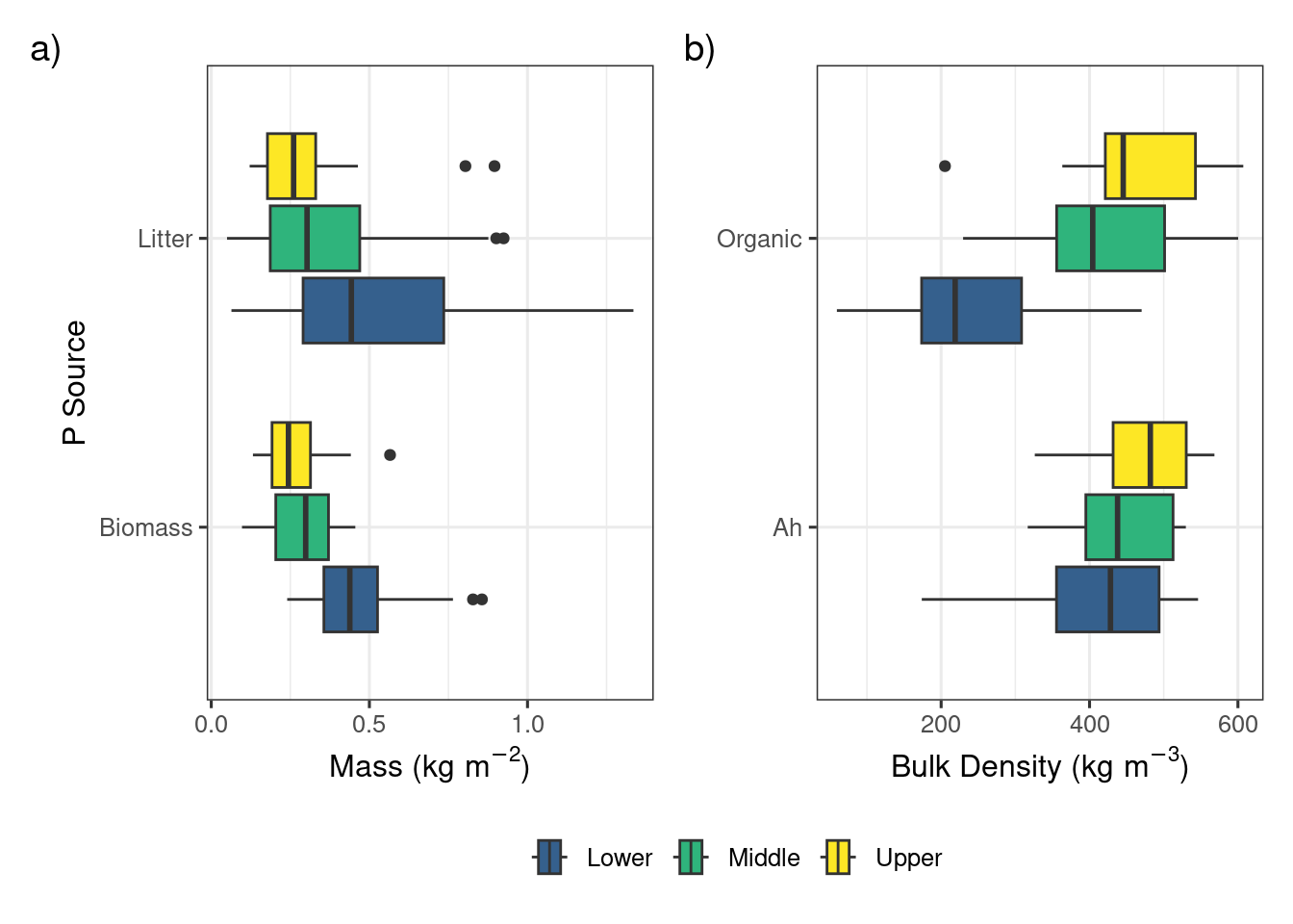
a) Mass of biomass and litter before grazing and mowing and b) the bulk density of the organic layer and 10 cm Ah horizon
In [8]:
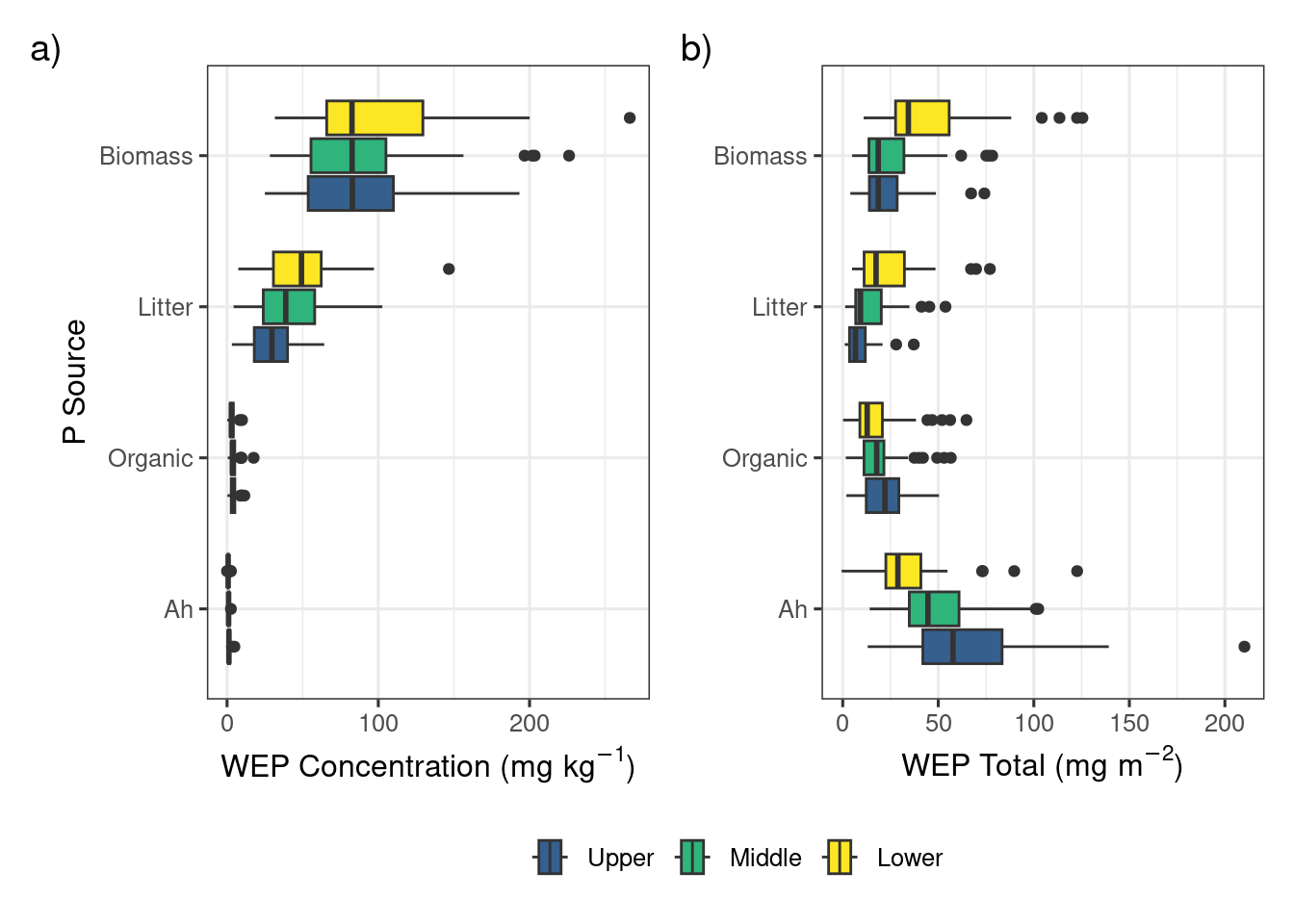
p1 <-ggplot(data = conc, aes(y = sample_type, x = conc, fill = location)) +geom_boxplot() +#scale_x_log10() +theme_bw(base_size =12) +theme(legend.position =c(0.2, 0.8),legend.title =element_blank()) +labs(x =expression(paste("WEP Concentration (", mg~kg^{-1}, ")")), y ="P Source", tag ="a)") +scale_fill_viridis_d(name ="Location", begin =0.3, end =1)
Warning: A numeric `legend.position` argument in `theme()` was deprecated in ggplot2
3.5.0.
ℹ Please use the `legend.position.inside` argument of `theme()` instead.
#p1p2 <-ggplot(data = total_data, aes(y = sample_type, x = p_total, fill = location)) +geom_boxplot() +#scale_x_log10() +theme_bw(base_size =12) +theme(axis.title.y =element_blank(),legend.position ="none") +labs(x =expression(paste("WEP Total (", mg~m^{-2}, ")")), tag ="b)") +scale_fill_viridis_d(name ="Location", begin =0.3, end =1)#p2