Riparian organic and mineral soil WEP in response to grazing

Load Libraries

In [1]:

library(tidyverse)

── Attaching core tidyverse packages ──────────────────────── tidyverse 2.0.0 ──
✔ dplyr     1.1.4     ✔ readr     2.1.5
✔ forcats   1.0.0     ✔ stringr   1.5.1
✔ ggplot2   3.5.1     ✔ tibble    3.2.1
✔ lubridate 1.9.3     ✔ tidyr     1.3.1
✔ purrr     1.0.2     
── Conflicts ────────────────────────────────────────── tidyverse_conflicts() ──
✖ dplyr::filter() masks stats::filter()
✖ dplyr::lag()    masks stats::lag()
ℹ Use the conflicted package (<http://conflicted.r-lib.org/>) to force all conflicts to become errors

library(glmmTMB)
library(DHARMa)

This is DHARMa 0.4.6. For overview type '?DHARMa'. For recent changes, type news(package = 'DHARMa')

library(emmeans)
library(gt)

Read in clean data

In [2]:

conc <- read_csv(here::here("./notebooks/P_concentration.csv")) %>%
  rename("conc" = "ak_content")

Rows: 1141 Columns: 8
── Column specification ────────────────────────────────────────────────────────
Delimiter: ","
chr (5): sample_type, timing, plot, location, treatment
dbl (3): site, ak_content, year

ℹ Use `spec()` to retrieve the full column specification for this data.
ℹ Specify the column types or set `show_col_types = FALSE` to quiet this message.

Organics data

In [3]:

organic_diff <- conc %>%
  filter(sample_type == "Organic") %>%
  pivot_wider(names_from = timing, values_from = conc) %>%
  mutate(diff = Before - After) %>%
  mutate(treatment = fct_recode(treatment, "Graze" = "Regular Graze")) %>%
  mutate(treatment = fct_relevel(treatment, c("Control", "Graze", "High Graze", "Mow"))) %>%
  mutate(location = fct_relevel(location, c("Upper", "Middle", "Lower")))

Soil data

In [4]:

soil_diff <- conc %>%
  filter(sample_type == "Soil") %>%
  pivot_wider(names_from = timing, values_from = conc) %>%
  mutate(diff = Before - After) %>%
  mutate(treatment = fct_recode(treatment, "Graze" = "Regular Graze")) %>%
  mutate(treatment = fct_relevel(treatment, c("Control", "Graze", "High Graze", "Mow"))) %>%
  mutate(location = fct_relevel(location, c("Upper", "Middle", "Lower")))

Organics analysis

In [5]:

m7 <- glmmTMB(diff ~ treatment * location + (1|site) + (1|year),
              data = organic_diff)

In [6]:

simulateResiduals(m7, n = 1000, plot = TRUE)

Object of Class DHARMa with simulated residuals based on 1000 simulations with refit = FALSE . See ?DHARMa::simulateResiduals for help. 
 
Scaled residual values: 0.238 0.027 0.226 0.24 0.719 0.392 0.179 0.09 0.368 0.246 0.39 0.748 0.864 0.689 0.362 0.796 0.846 0.507 0.995 0.711 ...

In [7]:

car::Anova(m7, type = "III")  # No interaction

Analysis of Deviance Table (Type III Wald chisquare tests)

Response: diff
                    Chisq Df Pr(>Chisq)
(Intercept)        0.0818  1     0.7748
treatment          3.4927  3     0.3217
location           0.4320  2     0.8058
treatment:location 2.8111  6     0.8322

In [8]:

m7 <- glmmTMB(diff ~ treatment + location + (1|site) + (1|year),
              data = organic_diff)
simulateResiduals(m7, n = 1000, plot = TRUE) # No interaction

Object of Class DHARMa with simulated residuals based on 1000 simulations with refit = FALSE . See ?DHARMa::simulateResiduals for help. 
 
Scaled residual values: 0.246 0.033 0.186 0.226 0.693 0.435 0.183 0.12 0.31 0.257 0.319 0.8 0.865 0.745 0.32 0.802 0.881 0.428 0.995 0.63 ...

performance::check_collinearity(m7)

# Check for Multicollinearity

Low Correlation

      Term  VIF      VIF  CI Increased SE Tolerance
 treatment 1.00 [1.00, 1.00]         1.00      1.00
  location 1.00 [1.00, 1.00]         1.00      1.00

car::Anova(m7, type = "III")

Analysis of Deviance Table (Type III Wald chisquare tests)

Response: diff
             Chisq Df Pr(>Chisq)  
(Intercept) 0.9723  1    0.32411  
treatment   8.2398  3    0.04131 *
location    0.5743  2    0.75039  
---
Signif. codes:  0 '***' 0.001 '**' 0.01 '*' 0.05 '.' 0.1 ' ' 1

Post-hoc

In [9]:

m_emms7 <- emmeans(m7, ~treatment)
pairs(m_emms7, adjust = "fdr")

 contrast             estimate    SE  df t.ratio p.value
 Control - Graze        -1.486 0.594 135  -2.501  0.0656
 Control - High Graze   -0.625 0.594 135  -1.052  0.3534
 Control - Mow          -1.378 0.594 135  -2.319  0.0656
 Graze - High Graze      0.861 0.594 135   1.449  0.2994
 Graze - Mow             0.108 0.594 135   0.182  0.8560
 High Graze - Mow       -0.753 0.594 135  -1.267  0.3110

Results are averaged over the levels of: location 
P value adjustment: fdr method for 6 tests 

location_pair <- summary(pairs(m_emms7, adjust = "fdr")) 

pairs <- location_pair %>%
  rename("Contrast" = "contrast", "Estimate" = "estimate", "t ratio" = "t.ratio", "p value" = "p.value")

In [10]:

In [11]:

pairs |>
  gt() |>
  fmt_number(columns = c("Estimate", "SE", "t ratio"), decimal = 2)|>
  fmt_number(columns = c("p value"), decimal = 3)|>
  sub_small_vals(threshold = 0.001) |>
  tab_style(style =  cell_text(weight = "bold", align = "center"), locations =  cells_row_groups()) |>
  tab_options(column_labels.font.weight = "bold")

Results of the post-hoc pairwise comparisons with a Benjamini-Hochberg p value adjustment for differences in the net organic layer WEP (\(mg~kg^{-1}\)) between the four treatments.

Contrast	Estimate	SE	df	t ratio	p value
Control - Graze	−1.49	0.59	135	−2.50	0.066
Control - High Graze	−0.63	0.59	135	−1.05	0.353
Control - Mow	−1.38	0.59	135	−2.32	0.066
Graze - High Graze	0.86	0.59	135	1.45	0.299
Graze - Mow	0.11	0.59	135	0.18	0.856
High Graze - Mow	−0.75	0.59	135	−1.27	0.311

Plots

Extra

In [12]:

df <- data.frame(x1 = c(-Inf, -Inf), x2 = c(Inf, Inf), y2 = c(Inf, 0), y1 = c(0, -Inf), difference = c("Net removal", "Net addition")) %>%
  mutate(difference = fct_relevel(difference, c("Net removal", "Net addition"))) 

Plots

In [13]:

#|
p1 <- ggplot(data = organic_diff) +
  theme_bw(base_size = 12) + 
  geom_rect(data = df, aes(xmin = x1, xmax = x2, ymin = y1, ymax = y2, fill = difference), alpha = 0.15) +
  #scale_fill_manual(values = c("white", "black")) +
  #ggnewscale::new_scale_fill() +
  geom_boxplot(aes(x = treatment, y = diff, fill = location)) +
  #scale_fill_viridis_d(name = "Location", begin = 0.3, end = 1) +
  scale_fill_manual(values = c("white", "black", "#35608DFF", "#2FB47CFF", "#FDE725FF")) +
  guides(fill = guide_legend(override.aes = list(colour = "black", size = 1))) +
  labs(y = expression(paste("Net WEP Difference (", mg~kg^{-1}, ")")), x = "Treatment") +
  theme(axis.title.x = element_blank(),
        axis.text.x = element_text(angle = 0, vjust = 1, hjust = 0.5),
        legend.position = 'bottom', legend.title = element_blank())
p1
#ggsave(plot = p1, filename = "Figures/Organics_WEP.png", width = 150, height = 100, units = "mm", dpi = 600)

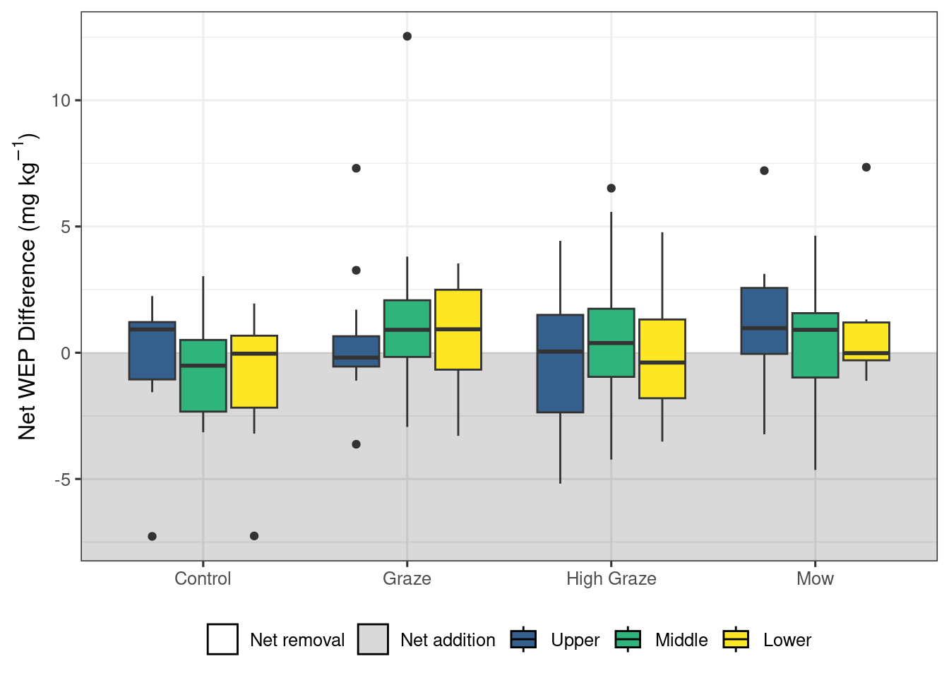
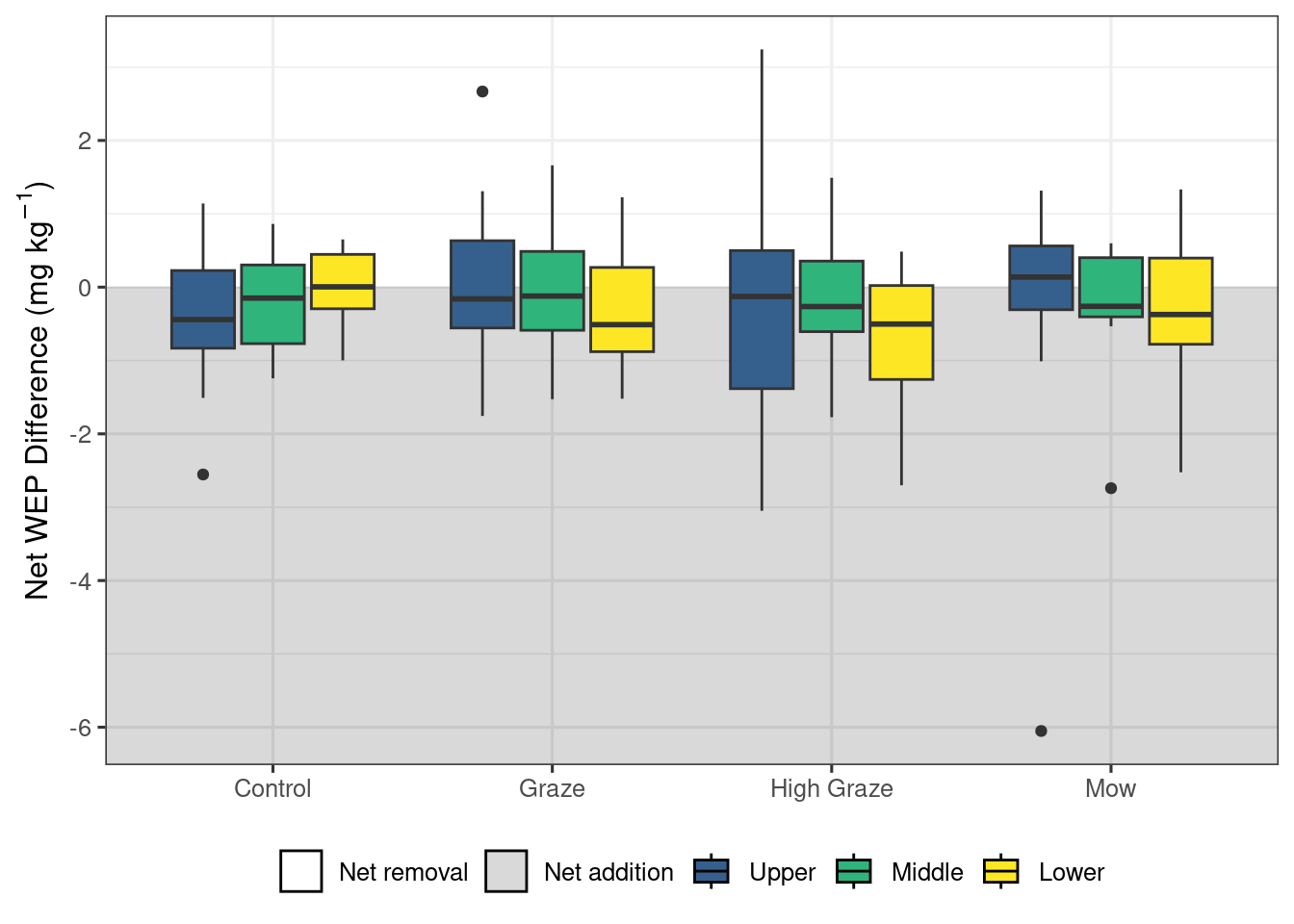
Change in riparian organic layer WEP concentration following grazing or mowing in each of the riparian locations. A significant effect of treatment was detected; however, the post-hoc analysis was not able to detect any significant (p < 0.05) pairwise contrasts. Lower sampling locations are adjacent to the edge of the waterbody and Upper locations are adjacent to the field.

Mineral soil analysis

In [14]:

m8 <- glmmTMB(diff ~ treatment * location + (1|site) + (1|year),
              data = soil_diff)
simulateResiduals(m8, n = 1000, plot = TRUE) 

Object of Class DHARMa with simulated residuals based on 1000 simulations with refit = FALSE . See ?DHARMa::simulateResiduals for help. 
 
Scaled residual values: 0.037 0.063 0.012 0.314 0.393 0.032 0.242 0.114 0.046 0.028 0.011 0 0.07 0.132 0.188 0.225 0.153 0.18 0.264 0.093 ...

car::Anova(m8, type = "III") # No interaction

Analysis of Deviance Table (Type III Wald chisquare tests)

Response: diff
                    Chisq Df Pr(>Chisq)
(Intercept)        0.7087  1     0.3999
treatment          1.8322  3     0.6080
location           1.0736  2     0.5846
treatment:location 4.3581  6     0.6283

No interaction

In [15]:

m8 <- glmmTMB(diff ~ treatment + location + (1|site) + (1|year),
              data = soil_diff)
simulateResiduals(m8, n = 1000, plot = TRUE) 

Object of Class DHARMa with simulated residuals based on 1000 simulations with refit = FALSE . See ?DHARMa::simulateResiduals for help. 
 
Scaled residual values: 0.021 0.08 0.014 0.389 0.363 0.018 0.219 0.111 0.06 0.03 0.011 0 0.065 0.158 0.27 0.203 0.114 0.123 0.311 0.121 ...

performance::check_collinearity(m8)

# Check for Multicollinearity

Low Correlation

      Term  VIF      VIF  CI Increased SE Tolerance
 treatment 1.00 [1.00, 1.00]         1.00      1.00
  location 1.00 [1.00, 1.00]         1.00      1.00

car::Anova(m8, type = "III")

Analysis of Deviance Table (Type III Wald chisquare tests)

Response: diff
             Chisq Df Pr(>Chisq)
(Intercept) 0.2055  1     0.6503
treatment   2.5924  3     0.4588
location    1.1674  2     0.5578

plots

In [16]:

#|
p2 <- ggplot(data = soil_diff) +
  theme_bw(base_size = 12) + 
  geom_rect(data = df, aes(xmin = x1, xmax = x2, ymin = y1, ymax = y2, fill = difference), alpha = 0.15) +
  #scale_fill_manual(values = c("white", "black")) +
  #ggnewscale::new_scale_fill() +
  geom_boxplot(aes(x = treatment, y = diff, fill = location)) +
  #scale_fill_viridis_d(name = "Location", begin = 0.3, end = 1) +
  scale_fill_manual(values = c("white", "black", "#35608DFF", "#2FB47CFF", "#FDE725FF")) +
  guides(fill = guide_legend(override.aes = list(colour = "black", size = 1))) +
  labs(y = expression(paste("Net WEP Difference (", mg~kg^{-1}, ")")), x = "Treatment") +
  theme(axis.title.x = element_blank(),
        axis.text.x = element_text(angle = 0, vjust = 1, hjust = 0.5),
        legend.position = 'bottom', legend.title = element_blank())
p2
#ggsave(plot = p2, filename = "Figures/Soil_WEP.png", width = 150, height = 100, units = "mm", dpi = 600)

Change in riparian Ah layer (0-10cm) WEP concentration following grazing or mowing in each of the riparian locations. No significant effect of treatment or location was detected. Lower sampling locations are adjacent to the edge of the waterbody and Upper locations are adjacent to the field.