Riparian litter WEP in response to grazing

Load Libraries

In [1]:

library(tidyverse)

── Attaching core tidyverse packages ──────────────────────── tidyverse 2.0.0 ──
✔ dplyr     1.1.4     ✔ readr     2.1.5
✔ forcats   1.0.0     ✔ stringr   1.5.1
✔ ggplot2   3.5.1     ✔ tibble    3.2.1
✔ lubridate 1.9.3     ✔ tidyr     1.3.1
✔ purrr     1.0.2     
── Conflicts ────────────────────────────────────────── tidyverse_conflicts() ──
✖ dplyr::filter() masks stats::filter()
✖ dplyr::lag()    masks stats::lag()
ℹ Use the conflicted package (<http://conflicted.r-lib.org/>) to force all conflicts to become errors

library(glmmTMB)
library(DHARMa)

This is DHARMa 0.4.6. For overview type '?DHARMa'. For recent changes, type news(package = 'DHARMa')

library(emmeans)
library(viridis)

Loading required package: viridisLite

library(patchwork)

Read in data

In [2]:

conc <- read_csv(here::here("./notebooks/P_concentration.csv"))

Rows: 1141 Columns: 8
── Column specification ────────────────────────────────────────────────────────
Delimiter: ","
chr (5): sample_type, timing, plot, location, treatment
dbl (3): site, ak_content, year

ℹ Use `spec()` to retrieve the full column specification for this data.
ℹ Specify the column types or set `show_col_types = FALSE` to quiet this message.

mass_data <- read_csv(here::here("./notebooks/mass.csv"))

Rows: 576 Columns: 8
── Column specification ────────────────────────────────────────────────────────
Delimiter: ","
chr (5): sample_type, timing, plot, location, treatment
dbl (3): site, dryweight, year

ℹ Use `spec()` to retrieve the full column specification for this data.
ℹ Specify the column types or set `show_col_types = FALSE` to quiet this message.

Merge data

In [3]:

veg_data <- mass_data %>%
  right_join(conc) %>%
  rename(conc = ak_content) %>% # mg/kg
  mutate(p_total = conc * dryweight/1000 /0.25) # mg/m2

Joining with `by = join_by(sample_type, site, timing, plot, location, year,
treatment)`

Litter data

In [4]:

litter_diff <- veg_data %>%
  filter(sample_type == "Litter") %>%
  mutate(dryweight = dryweight/1000 /0.25) %>%
  pivot_longer(cols = c(dryweight, p_total, conc), names_to = "measure", values_to = "value") %>%
  pivot_wider(names_from = timing, values_from = value) %>%
  mutate(diff = Before - After) 

Litter Analysis

P-total

In [5]:

m4 <- glmmTMB(diff ~ treatment * location + (1|site) + (1|year),
             data = filter(litter_diff, measure == "p_total"))
simulateResiduals(m4, n = 1000, plot = TRUE) 

Object of Class DHARMa with simulated residuals based on 1000 simulations with refit = FALSE . See ?DHARMa::simulateResiduals for help. 
 
Scaled residual values: 0.78 0.652 0.998 0.43 0.789 0.365 0.765 0.871 0.046 0.873 0.903 0.276 0.639 0.764 1 0.845 0.556 0.028 0.655 0.815 ...

car::Anova(m4, type = "III") # No interaction

Analysis of Deviance Table (Type III Wald chisquare tests)

Response: diff
                    Chisq Df Pr(>Chisq)  
(Intercept)        2.8104  1    0.09366 .
treatment          2.3626  3    0.50064  
location           2.4069  2    0.30015  
treatment:location 3.3583  6    0.76271  
---
Signif. codes:  0 '***' 0.001 '**' 0.01 '*' 0.05 '.' 0.1 ' ' 1

Removing interaction

In [6]:

temp4 <- filter(litter_diff, measure == "p_total") ## otherwise issue with emmeans()
m4 <- glmmTMB(diff ~ treatment + location + (1|site) + (1|year),
             data = temp4)
simulateResiduals(m4, n = 1000, plot = TRUE)

Object of Class DHARMa with simulated residuals based on 1000 simulations with refit = FALSE . See ?DHARMa::simulateResiduals for help. 
 
Scaled residual values: 0.773 0.556 0.999 0.475 0.824 0.268 0.697 0.896 0.053 0.886 0.883 0.291 0.576 0.791 1 0.842 0.469 0.046 0.675 0.788 ...

performance::check_collinearity(m4)

# Check for Multicollinearity

Low Correlation

      Term  VIF  VIF 95% CI Increased SE Tolerance Tolerance 95% CI
 treatment 1.00 [1.00, Inf]         1.00      1.00     [0.00, 1.00]
  location 1.00 [1.00, Inf]         1.00      1.00     [0.00, 1.00]

car::Anova(m4, type = "III") # No sig impact of treatment or position

Analysis of Deviance Table (Type III Wald chisquare tests)

Response: diff
             Chisq Df Pr(>Chisq)
(Intercept) 0.9539  1     0.3287
treatment   4.3023  3     0.2306
location    1.1541  2     0.5615

Summary

In [7]:

litter_diff %>%
  filter(measure == "p_total") %>%
  group_by(treatment) %>%
  summarise(median = median(diff, na.rm =T),
            mean = mean(diff, na.rm =T))

# A tibble: 4 × 3
  treatment     median  mean
  <chr>          <dbl> <dbl>
1 Control        -1.05 -2.22
2 High Graze     -1.39 -2.36
3 Mow            -5.70 -7.94
4 Regular Graze  -1.66 -6.05

litter_diff %>%
  filter(measure == "p_total") %>%
  group_by(location) %>%
  summarise(median = median(diff, na.rm =T),
            mean = mean(diff, na.rm =T))

# A tibble: 3 × 3
  location median  mean
  <chr>     <dbl> <dbl>
1 Lower     -5.88 -5.53
2 Middle    -2.44 -5.56
3 Upper     -1.22 -2.72

Plots

Reorder factors

In [8]:

plot_data <- litter_diff %>% 
  mutate(treatment = fct_recode(treatment, "Graze" = "Regular Graze")) %>%
  mutate(treatment = fct_relevel(treatment, c("Control", "Graze", "High Graze", "Mow"))) %>%
  mutate(location = fct_relevel(location, c("Upper", "Middle", "Lower")))

Extra

In [9]:

df <- data.frame(x1 = c(-Inf, -Inf), x2 = c(Inf, Inf), y2 = c(Inf, 0), y1 = c(0, -Inf), difference = c("Net removal", "Net addition")) %>%
  mutate(difference = fct_relevel(difference, c("Net removal", "Net addition"))) 

Plots

In [10]:

#|
p1 <- ggplot(data = filter(plot_data, measure == "p_total")) +
  theme_bw(base_size = 12) +
  geom_rect(data = df, aes(xmin = x1, xmax = x2, ymin = y1, ymax = y2, fill = difference), alpha = 0.15) +
  #scale_fill_manual(values = c("white", "black")) +
  #ggnewscale::new_scale_fill() +
  geom_boxplot(aes(x = treatment, y = diff, fill = location)) +
  labs(y = expression(paste("Net WEP Difference (", mg~m^{-2}, ")")), x = "Treatment") +
  #scale_fill_viridis_d(name = "Location", begin = 0.3, end = 1) +
  scale_fill_manual(values = c("white", "black", "#35608DFF", "#2FB47CFF", "#FDE725FF")) +
  guides(fill = guide_legend(override.aes = list(colour = "black", size = 1))) +
  theme(axis.title.x = element_blank(),
        axis.text.x = element_text(angle = 0, vjust = 1, hjust = 0.5),
        legend.position = "bottom",
        legend.title = element_blank())
p1

Warning: Removed 11 rows containing non-finite outside the scale range
(`stat_boxplot()`).

#|
#ggsave(plot = p1, filename = "Figures/Litter_WEP.png", width = 150, height = 100, units = "mm", dpi = 600)

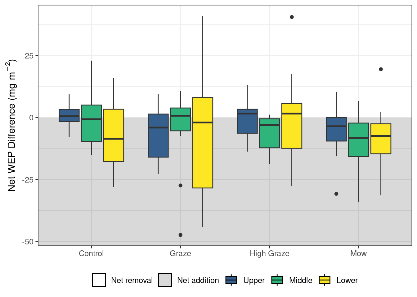
Change in riparian litter WEP following grazing or mowing in each of the riparian locations. No significant effect of treatment or riparian location on the litter WEP content was detected. Lower sampling locations are adjacent to the edge of the waterbody and Upper locations are adjacent to the field.