Riparian vegetation WEP in response to grazing

Load Libraries

In [1]:

library(tidyverse)

── Attaching core tidyverse packages ──────────────────────── tidyverse 2.0.0 ──
✔ dplyr     1.1.4     ✔ readr     2.1.5
✔ forcats   1.0.0     ✔ stringr   1.5.1
✔ ggplot2   3.5.1     ✔ tibble    3.2.1
✔ lubridate 1.9.3     ✔ tidyr     1.3.1
✔ purrr     1.0.2     
── Conflicts ────────────────────────────────────────── tidyverse_conflicts() ──
✖ dplyr::filter() masks stats::filter()
✖ dplyr::lag()    masks stats::lag()
ℹ Use the conflicted package (<http://conflicted.r-lib.org/>) to force all conflicts to become errors

library(glmmTMB)
library(DHARMa)

This is DHARMa 0.4.6. For overview type '?DHARMa'. For recent changes, type news(package = 'DHARMa')

library(emmeans)
library(viridis)

Loading required package: viridisLite

library(patchwork)
library(gt)

Read in data

In [2]:

conc <- read_csv(here::here("./notebooks/P_concentration.csv"))

Rows: 1141 Columns: 8
── Column specification ────────────────────────────────────────────────────────
Delimiter: ","
chr (5): sample_type, timing, plot, location, treatment
dbl (3): site, ak_content, year

ℹ Use `spec()` to retrieve the full column specification for this data.
ℹ Specify the column types or set `show_col_types = FALSE` to quiet this message.

mass_data <- read_csv(here::here("./notebooks/mass.csv"))

Rows: 576 Columns: 8
── Column specification ────────────────────────────────────────────────────────
Delimiter: ","
chr (5): sample_type, timing, plot, location, treatment
dbl (3): site, dryweight, year

ℹ Use `spec()` to retrieve the full column specification for this data.
ℹ Specify the column types or set `show_col_types = FALSE` to quiet this message.

Merge data

In [3]:

veg_data <- mass_data %>%
  right_join(conc) %>%
  rename(conc = ak_content) %>% # mg/kg
  mutate(p_total = conc * dryweight/1000 /0.25) # mg/m2

Joining with `by = join_by(sample_type, site, timing, plot, location, year,
treatment)`

Biomass data

In [4]:

biomass_diff <- veg_data %>%
  filter(sample_type == "Biomass") %>%
  mutate(dryweight = dryweight/1000 /0.25) %>% # kg/m2
  pivot_longer(cols = c(dryweight, p_total, conc), names_to = "measure", values_to = "value") %>%
  pivot_wider(names_from = timing, values_from = value) %>%
  mutate(diff = Before - After)

Biomass Analysis

P-total

In [5]:

m <- glmmTMB((diff) ~ treatment * location + Before + (1|site) + (1|year),
             data = filter(biomass_diff, measure == "p_total"))
simulateResiduals(m, n = 1000, plot = TRUE) 

Object of Class DHARMa with simulated residuals based on 1000 simulations with refit = FALSE . See ?DHARMa::simulateResiduals for help. 
 
Scaled residual values: 0.751 0.611 0.716 0.648 0.463 0.707 0.684 0.558 0.811 0.623 0.328 0.664 0.676 0.595 0.785 0.304 0.68 0.547 0.369 0.329 ...

car::Anova(m, type = "III") # No interaction

Analysis of Deviance Table (Type III Wald chisquare tests)

Response: (diff)
                      Chisq Df Pr(>Chisq)    
(Intercept)         22.1909  1  2.468e-06 ***
treatment           15.4435  3   0.001474 ** 
location             9.0047  2   0.011083 *  
Before             178.7862  1  < 2.2e-16 ***
treatment:location   6.3738  6   0.382650    
---
Signif. codes:  0 '***' 0.001 '**' 0.01 '*' 0.05 '.' 0.1 ' ' 1

Removing interaction

In [6]:

temp <- filter(biomass_diff, measure == "p_total") ## otherwise issue with emmeans()
m <- glmmTMB((diff) ~ treatment + location + Before + (1|site) + (1|year),
             data = temp)
simulateResiduals(m, n = 1000, plot = TRUE)

Object of Class DHARMa with simulated residuals based on 1000 simulations with refit = FALSE . See ?DHARMa::simulateResiduals for help. 
 
Scaled residual values: 0.781 0.692 0.617 0.69 0.469 0.664 0.714 0.47 0.829 0.472 0.332 0.78 0.71 0.511 0.803 0.336 0.739 0.442 0.245 0.323 ...

performance::check_collinearity(m)

# Check for Multicollinearity

Low Correlation

      Term  VIF       VIF 95% CI Increased SE Tolerance Tolerance 95% CI
 treatment 1.00 [1.00, 2.67e+11]         1.00      1.00     [0.00, 1.00]
  location 1.59 [1.33,     2.03]         1.26      0.63     [0.49, 0.75]
    Before 1.59 [1.34,     2.04]         1.26      0.63     [0.49, 0.75]

car::Anova(m, type = "III")

Analysis of Deviance Table (Type III Wald chisquare tests)

Response: (diff)
              Chisq Df Pr(>Chisq)    
(Intercept)  24.370  1  7.949e-07 ***
treatment    24.771  3  1.724e-05 ***
location     15.741  2  0.0003818 ***
Before      176.833  1  < 2.2e-16 ***
---
Signif. codes:  0 '***' 0.001 '**' 0.01 '*' 0.05 '.' 0.1 ' ' 1

Post-hoc

In [7]:

m_emms1 <- emmeans(m, ~treatment)
m_emms2 <- emmeans(m, ~location)

treat_pair <- summary(pairs(m_emms1, adjust = "fdr")) %>%
  mutate(type = "Treatment")
location_pair <- summary(pairs(m_emms2, adjust = "fdr")) %>%
  mutate(type = "Location")

pairs <- treat_pair %>%
  bind_rows(location_pair) %>%
  rename("Contrast" = "contrast", "Estimate" = "estimate", "t ratio" = "t.ratio", "p value" = "p.value")

In [8]:

In [9]:

pairs |>
  mutate(Contrast = fct_recode(Contrast, "Control - Graze" = "Control - Regular Graze", "High Graze - Graze" = "High Graze - Regular Graze", "Mow - Graze" = "Mow - Regular Graze")) |>
  group_by(type) |>
  gt() |>
  fmt_number(columns = c("Estimate", "SE", "t ratio"), decimal = 2)|>
  fmt_number(columns = c("p value"), decimal = 3)|>
  sub_small_vals(threshold = 0.001) |>
  tab_style(style =  cell_text(weight = "bold", align = "center"), locations =  cells_row_groups()) |>
  tab_options(column_labels.font.weight = "bold")

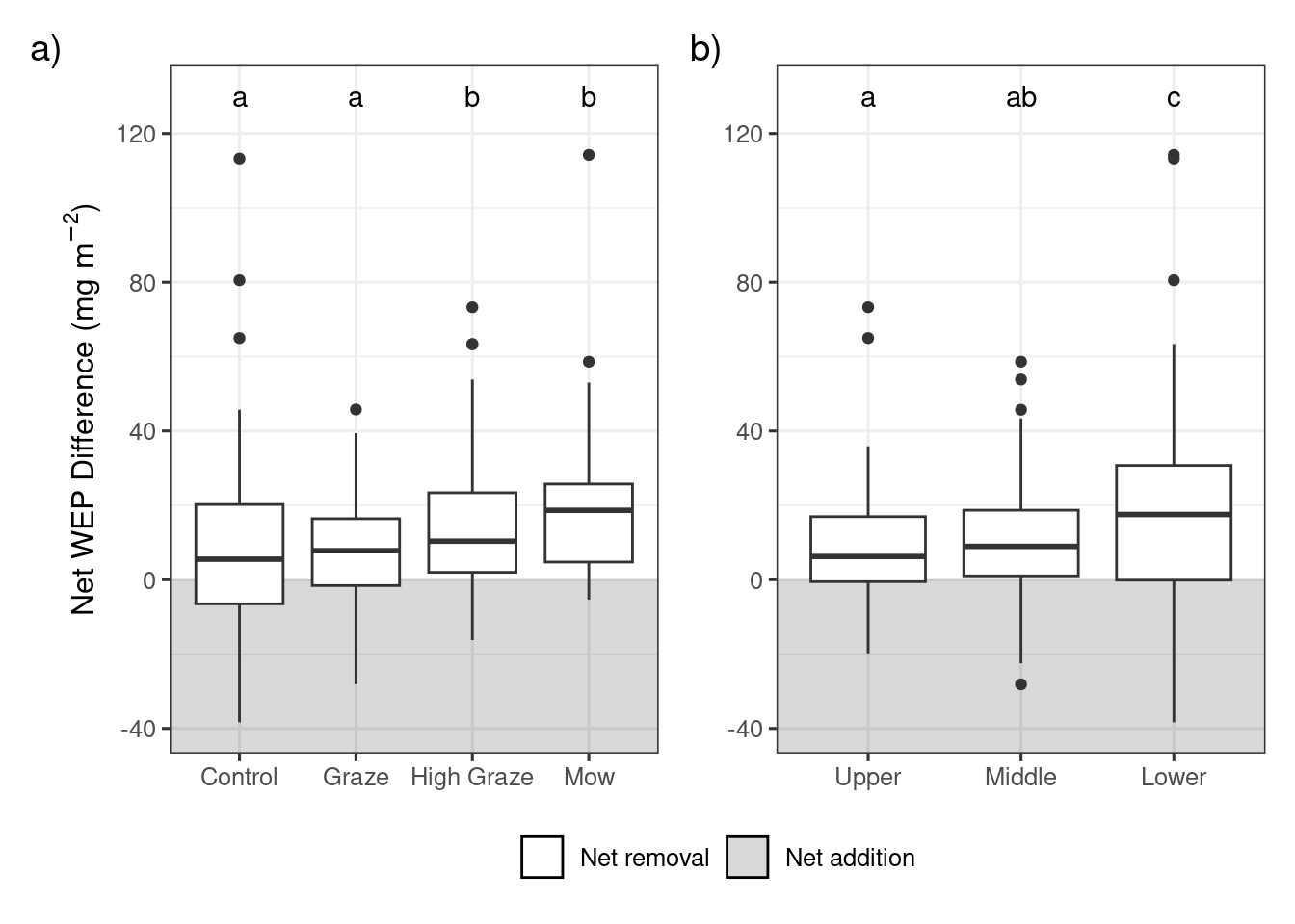
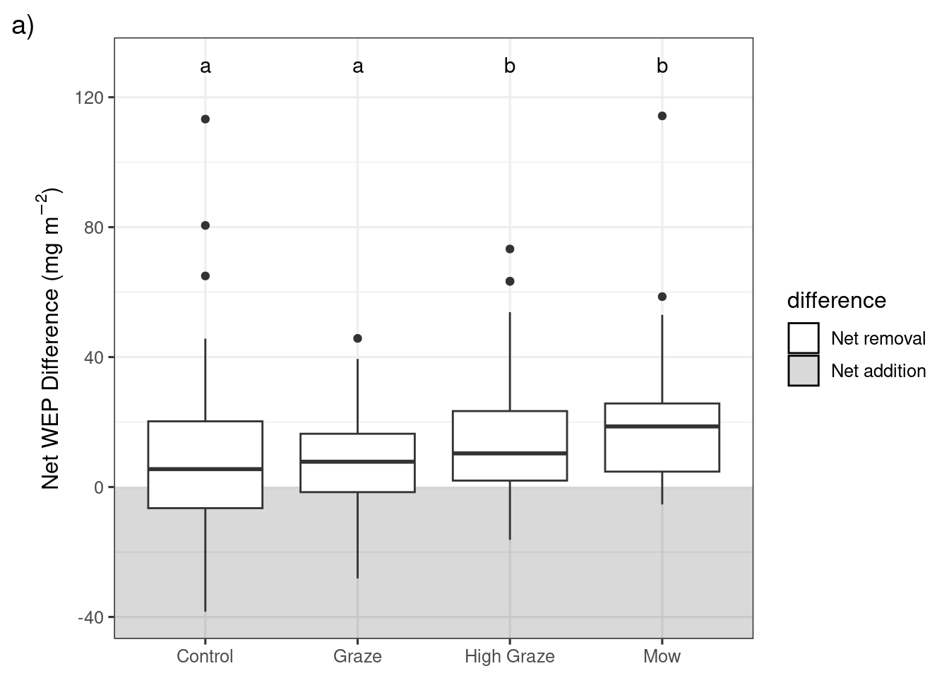
Results of the post-hoc pairwise comparisons with a Benjamini-Hochberg p value adjustment for differences in the net biomass WEP (\(mg~m^{-2}\)) between the four treatments and three riparian sampling locations.

Contrast	Estimate	SE	df	t ratio	p value
Treatment
Control - High Graze	−4.83	2.42	132	−2.00	0.072
Control - Mow	−8.52	2.42	132	−3.52	0.002
Control - Graze	2.47	2.40	132	1.03	0.306
High Graze - Mow	−3.69	2.43	132	−1.51	0.159
High Graze - Graze	7.30	2.42	132	3.02	0.006
Mow - Graze	10.99	2.42	132	4.55	<0.001
Location
Lower - Middle	−7.94	2.43	132	−3.26	0.002
Lower - Upper	−9.82	2.57	132	−3.83	<0.001
Middle - Upper	−1.87	2.11	132	−0.89	0.377

Summary

In [10]:

biomass_diff %>%
  filter(measure == "p_total") %>%
  group_by(treatment) %>%
  summarise(median = median(diff, na.rm =T),
            mean = mean(diff, na.rm =T))

# A tibble: 4 × 3
  treatment     median  mean
  <chr>          <dbl> <dbl>
1 Control         5.50 12.1 
2 High Graze     10.4  16.3 
3 Mow            18.7  19.5 
4 Regular Graze   7.79  7.64

biomass_diff %>%
  filter(measure == "p_total") %>%
  group_by(location) %>%
  summarise(median = median(diff, na.rm =T),
            mean = mean(diff, na.rm =T))

# A tibble: 3 × 3
  location median  mean
  <chr>     <dbl> <dbl>
1 Lower     17.5  20.1 
2 Middle     8.95 11.4 
3 Upper      6.23  9.89

Plotting

Ordering of factors

In [11]:

plot_data <- biomass_diff %>% 
  mutate(treatment = fct_recode(treatment, "Graze" = "Regular Graze")) %>%
  mutate(treatment = fct_relevel(treatment, c("Control", "Graze", "High Graze", "Mow"))) %>%
  mutate(location = fct_relevel(location, c("Upper", "Middle", "Lower")))

Extra

In [12]:

df <- data.frame(x1 = c(-Inf, -Inf), x2 = c(Inf, Inf), y2 = c(Inf, 0), y1 = c(0, -Inf), difference = c("Net removal", "Net addition")) %>%
  mutate(difference = fct_relevel(difference, c("Net removal", "Net addition"))) 

Plots

In [13]:

p1 <- ggplot(data = filter(plot_data, measure == "p_total")) +
  geom_rect(data = df, aes(xmin = x1, xmax = x2, ymin = y1, ymax = y2, fill = difference), alpha = 0.15) +
  #geom_hline(yintercept = 0) +
  scale_y_continuous(breaks = seq(-40, 120, 40)) +
  geom_boxplot(data = filter(plot_data, measure == "p_total"), aes(x = treatment, y = diff)) +
  theme_bw(base_size = 12) + 
  labs(y = expression(paste("Net WEP Difference (", mg~m^{-2}, ")")), x = "Treatment", tag = "a)") +
  annotate("text", x = "Control", y = 130, label = "a") + 
  annotate("text", x = "Graze", y = 130, label = "a") + 
  annotate("text", x = "High Graze", y = 130, label = "b") + 
  annotate("text", x = "Mow", y = 130, label = "b") +
  scale_fill_manual(values = c("white", "black"), guide = guide_legend(override.aes = list(colour = "black"))) +
  theme(axis.title.x = element_blank(),
        axis.text.x = element_text(angle = 0, vjust = 1, hjust = 0.5))
p1

Warning: Removed 2 rows containing non-finite outside the scale range
(`stat_boxplot()`).

p2 <- ggplot() +
  geom_rect(data = df, aes(xmin = x1, xmax = x2, ymin = y1, ymax = y2, fill = difference), alpha = 0.15) +
  geom_boxplot(data = filter(plot_data, measure == "p_total"), aes(x = location, y = diff)) +
  theme_bw(base_size = 12) + 
  scale_y_continuous(breaks = seq(-40, 120, 40)) +
  labs(tag = "b)") +
  annotate("text", x = "Upper", y = 130, label = "a") + 
  annotate("text", x = "Middle", y = 130, label = "ab") + 
  annotate("text", x = "Lower", y = 130, label = "c") +
  scale_fill_manual(values = c("white", "black"), guide = guide_legend(override.aes = list(colour = "black"))) +
  theme(axis.title.y = element_blank(),
        axis.title.x = element_blank(),
        axis.text.x = element_text(angle = 0, vjust = 1, hjust = 0.5))
p2

Warning: Removed 2 rows containing non-finite outside the scale range
(`stat_boxplot()`).

In [14]:

#|
p3 <- p1 + p2 + plot_layout(guides = 'collect') & theme(legend.position = 'bottom', legend.title = element_blank())
p3

Warning: Removed 2 rows containing non-finite outside the scale range
(`stat_boxplot()`).
Removed 2 rows containing non-finite outside the scale range
(`stat_boxplot()`).

#|
# ggsave(plot = p3, filename = "Figures/Biomass_WEP.png", width = 174, height = 85, units = "mm", dpi = 600)

Change in riparian biomass WEP following grazing or mowing in each riparian location. Within each plot significant differences (p<0.05) between treatments or riparian locations are denoted with different letters. Lower sampling locations are adjacent to the edge of the waterbody and Upper locations are adjacent to the field.

Dry Weight

In [15]:

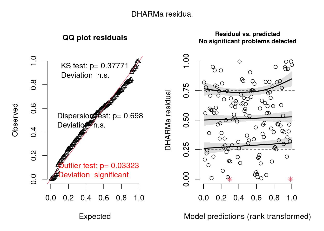
m2 <- glmmTMB((diff) ~ treatment * location + Before + (1|site) + (1|year),
              data = filter(biomass_diff, measure == "dryweight"))
simulateResiduals(m2, n = 1000, plot = TRUE)

Object of Class DHARMa with simulated residuals based on 1000 simulations with refit = FALSE . See ?DHARMa::simulateResiduals for help. 
 
Scaled residual values: 0.854 0.648 0.326 0.646 0.318 0.725 0.668 0.466 0.81 0.586 0.427 0.882 0.777 0.897 0.805 0.368 0.704 0.594 0.586 0.522 ...

car::Anova(m2, type = "III")

Analysis of Deviance Table (Type III Wald chisquare tests)

Response: (diff)
                    Chisq Df Pr(>Chisq)    
(Intercept)        26.264  1  2.978e-07 ***
treatment          14.420  3   0.002385 ** 
location           10.771  2   0.004581 ** 
Before             76.432  1  < 2.2e-16 ***
treatment:location 13.564  6   0.034909 *  
---
Signif. codes:  0 '***' 0.001 '**' 0.01 '*' 0.05 '.' 0.1 ' ' 1

performance::check_collinearity(glmmTMB((diff) ~ treatment + location + Before + (1|site) + (1|year),
                                        data = filter(biomass_diff, measure == "dryweight")))

# Check for Multicollinearity

Low Correlation

      Term  VIF   VIF 95% CI Increased SE Tolerance Tolerance 95% CI
 treatment 1.04 [1.00, 2.88]         1.02      0.96     [0.35, 1.00]
  location 1.77 [1.47, 2.27]         1.33      0.57     [0.44, 0.68]
    Before 1.81 [1.50, 2.32]         1.35      0.55     [0.43, 0.67]

Post-hoc

In [16]:

m_emms2 <- emmeans(m2, ~treatment * location)
emmeans(m2, pairwise ~ location|treatment, adjust = "fdr")$contrasts

treatment = Control:
 contrast       estimate     SE  df t.ratio p.value
 Lower - Middle -0.03993 0.0395 128  -1.011  0.3138
 Lower - Upper  -0.12232 0.0389 128  -3.147  0.0062
 Middle - Upper -0.08239 0.0365 128  -2.257  0.0386

treatment = High Graze:
 contrast       estimate     SE  df t.ratio p.value
 Lower - Middle -0.12667 0.0382 128  -3.315  0.0018
 Lower - Upper  -0.14328 0.0383 128  -3.744  0.0008
 Middle - Upper -0.01661 0.0365 128  -0.456  0.6495

treatment = Mow:
 contrast       estimate     SE  df t.ratio p.value
 Lower - Middle -0.02560 0.0372 128  -0.689  0.7859
 Lower - Upper  -0.01067 0.0392 128  -0.272  0.7859
 Middle - Upper  0.01493 0.0372 128   0.401  0.7859

treatment = Regular Graze:
 contrast       estimate     SE  df t.ratio p.value
 Lower - Middle  0.00666 0.0411 128   0.162  0.8716
 Lower - Upper  -0.02837 0.0430 128  -0.660  0.7658
 Middle - Upper -0.03503 0.0367 128  -0.955  0.7658

Note: contrasts are still on the ( scale 
P value adjustment: fdr method for 3 tests 

emmeans(m2, pairwise ~ treatment|location, adjust = "fdr")$contrasts

location = Lower:
 contrast                   estimate     SE  df t.ratio p.value
 Control - High Graze        -0.0674 0.0368 128  -1.829  0.1046
 Control - Mow               -0.1391 0.0368 128  -3.778  0.0014
 Control - Regular Graze     -0.0532 0.0368 128  -1.446  0.1808
 High Graze - Mow            -0.0717 0.0365 128  -1.966  0.1029
 High Graze - Regular Graze   0.0142 0.0378 128   0.375  0.7081
 Mow - Regular Graze          0.0859 0.0378 128   2.274  0.0740

location = Middle:
 contrast                   estimate     SE  df t.ratio p.value
 Control - High Graze        -0.1541 0.0365 128  -4.222  0.0003
 Control - Mow               -0.1248 0.0366 128  -3.410  0.0017
 Control - Regular Graze     -0.0066 0.0365 128  -0.181  0.8567
 High Graze - Mow             0.0294 0.0367 128   0.799  0.5107
 High Graze - Regular Graze   0.1475 0.0366 128   4.036  0.0003
 Mow - Regular Graze          0.1182 0.0365 128   3.235  0.0023

location = Upper:
 contrast                   estimate     SE  df t.ratio p.value
 Control - High Graze        -0.0883 0.0366 128  -2.412  0.0518
 Control - Mow               -0.0274 0.0370 128  -0.743  0.4591
 Control - Regular Graze      0.0408 0.0367 128   1.109  0.3234
 High Graze - Mow             0.0609 0.0366 128   1.665  0.1474
 High Graze - Regular Graze   0.1291 0.0365 128   3.538  0.0034
 Mow - Regular Graze          0.0682 0.0365 128   1.868  0.1280

Note: contrasts are still on the ( scale 
P value adjustment: fdr method for 6 tests 

Plots

In [17]:

ggplot(data = filter(plot_data, measure == "dryweight"), aes(x = treatment, y = diff, fill = location)) +
  geom_boxplot() +
  labs(y = "kg/m^2") +
  geom_hline(yintercept = 0) +
  facet_grid(~measure) 

ggplot(data = filter(plot_data, measure == "dryweight"), aes(x = treatment, y = diff, fill = location)) +
  geom_boxplot() +
  labs(y = "kg/m^2") +
  geom_hline(yintercept = 0) +
  facet_grid(location~measure) 

ggplot(data = filter(plot_data, measure == "dryweight"), aes(x = location, y = diff, fill = treatment)) +
  geom_boxplot() +
  labs(y = "kg/m^2") +
  geom_hline(yintercept = 0) +
  facet_grid(treatment~measure)