p6 <- p4 + inset_element(p1, left = 0.6, bottom = 0.6, right = 1, top = 1) + p5
p6
Warning in st_point_on_surface.sfc(sf::st_zm(x)): st_point_on_surface may not
give correct results for longitude/latitude data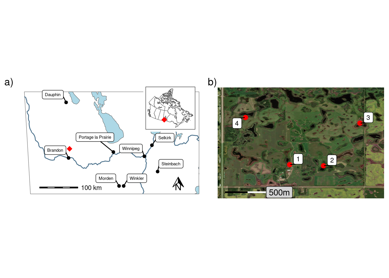
Riparian areas play an important role in maintaining water quality in agricultural watersheds by buffering sediment, nutrients, and other pollutants. Recent studies have shown that in some cases riparian areas are a net source of phosphorus (P) in cold climates. This study assessed the impact of cattle grazing or harvesting of riparian areas on the spatial and vertical distribution of water-extractable phosphorus (WEP). This study measured the WEP in four distinctive sources: biomass, litter, organic layer, and Ah horizon in three riparian locations extending from the edge of the waterbody to the field edge. In addition to a control, three treatments were examined: 1) grazing; 2) high-density grazing; and 3) mowing. Prior to implementing the treatments, the Ah (0-10cm) soil was the largest pool of WEP (42.5 mg m-2, ~44%); however, the biomass (i.e., standing vegetation) was a considerable proportion of the total (26.3 mg m-2, ~25%) WEP pool. The litter and organic layer had median WEP areal densities of 11.1 and 17.7 mg m-2, respectively. Findings revealed significant reductions in biomass WEP with median reductions of 10.4 and 18.7 mg m-2 for high-density grazing and mowing treatments, respectively. This reduction was more pronounced in the lower riparian locations where there was more biomass available to be grazed or mowed. There were no detectable changes in the other sources of WEP across all the treatments. Assessment of the control plots (pre- and post-treatment) clearly indicate that there is considerable small-scale spatial variability in P measurements in riparian areas. Overall, the results of this study suggest that management practices that target vegetation, including harvesting and autumn short-term grazing, may be mechanisms to reduce the potential P loss during the snowmelt period. To fully assess the risk of P loss, studies investigating other important riparian processes that also have a demonstrated impact on P mobility, including freeze-thaw cycles and flooding, are needed.
Phosphorus, Grazing, Riparian
Core ideas
Abbreviations
MBFI, Manitoba Beef and Forage Initiatives; P, phosphorus; WEP, water extractable phosphorus
The increasing frequency and extent of algal blooms is typically linked to increased nutrient loading into lake and rivers. Phosphorus (P) loading is particularly concerning as this is generally the limiting nutrient in freshwater systems (Schindler et al., 2012). There have been many lab and field studies demonstrating the role and functionality of riparian areas in reducing P loading to surface water in agricultural settings (Yu et al., 2019). Infiltration, adsorption, biological uptake, microbial activity, and sedimentation are the key processes that intercept and buffer the delivery of P (Lacas et al., 2005; Owens et al., 2007; McGuire and McDonnell, 2010).Convergence within the landscape coupled with climatic/weather conditions creates variability in hydrologic conditions and pathways, reducing the buffering capacity of riparian areas and ultimately resulting in reduced, inconsistent, and/or unsustainable reductions in P loading relative to many controlled experimental studies (Roberts et al., 2012; Habibiandehkordi et al., 2017).
In cold climates, the reduced infiltration due to frozen ground, limited vegetation uptake, and low microbial activity coupled with a flashy hydrograph hydrograph (rapid rise and fall in discharge) during snowmelt creates conditions that further compromise the buffering capacity of riparian areas (Kieta et al., 2018; Nsenga Kumwimba et al., 2023). Additionally, research increasingly shows that riparian areas can contribute P (i.e., net source) from soil and vegetation to the surrounding environment (Roberts et al., 2012). As soil P concentration increases, so does the risk of P loss through leaching and runoff (Habibiandehkordi et al., 2019). Soil P release can be intensified during periods of inundation that often occur during the spring snow melt, due to both to a longer period of soil-water contact and an increased solubility of iron-bound P as soil redox conditions lower (i.e., become anaerobic) (Carlyle and Hill, 2001; Young and Briggs, 2008). Vegetation P can become more mobile through the mineralization of P from decaying vegetation near the soil surface. There is also evidence that the longer vegetation-water contact during periods of inundation will also increase the mass of P leached out of the dead vegetation and contribute to the P available to be lost during runoff (Lozier and Macrae, 2017; Liu et al., 2019b). Both the soil and vegetation P sources can also be affected by freeze-thaw cycles. Repeated freeze-thaw cycles result in the cell disruption of microbial and plant biomass, releasing inter-cellular P to the surrounding environment (Kieta and Owens, 2019).
Management of riparian areas to maintain or enhance the buffering capacity of P is typically needed to prevent loss to water bodies. Unlike nitrogen (N), which can be significantly lost to the atmosphere through nitrification and denitrification to offset the continued input (Lyu et al., 2021), when not taken up by plants, P is generally only lost through runoff or leaching. Harvesting and removing of biomass from the riparian area for use as forage can be a practice to remove P. Mechanized biomass harvesting may be impractical or unsafe due to steep gradients, wet soil, and other obstacles like trees; however, livestock grazing in riparian areas (riparian pastures) is common in the Canadian Prairies due to the abundance of forage, particularly during drought. Livestock exclusion from riparian areas has been suggested as a best management practice to reduce the direct inputs of P, limit bank erosion, and avoid soil compaction (Krall and Roni, 2023). However, strategies including alternative water sources, rotational grazing, timed-controlled grazing, rest-rotation grazing, and corridor fencing can all reduce those risks (Fitch et al., 2003).
From a surface water quality perspective, understanding the near-surface P distribution, both vertically and longitudinally, will help develop and identify best management practices for reducing P loading from riparian areas. Vertically, there are often four distinctive and identifiable sources of near-surface P: 1) biomass consisting of living standing vegetation; 2) litter consisting of fresh (within the first three years) residues; 3) partially to well-decomposed organic material; and 4) mineral soil (Reid et al., 2018). Longitudinally there often is a strong soil moisture gradient extending from the edge of the waterbody to the field edge. This results in changes in the mass and composition of biomass and litter as well as soil properties including organic matter content and horizon thickness. A better understanding of the spatial variability and relative contributions of the different sources of P is is helpful in building a more complete representation of riparian processes and function.
Given the timing and processes of P dynamics within riparian areas in cold climates, like the Canadian Prairies, reducing the near-surface concentration of soluble P prior to spring snowmelt could be a strategy to limit the contribution of P from the riparian area to surface water. Therefore, the overall aim of this study is to assess the impacts of short-term autumn cattle grazing and mowing on the sources and distribution of P in riparian areas. The objectives of this study were to quantify 1) the vertical profile of WEP using four distinctive P sources: biomass, litter, organic layer, and Ah horizon; 2) each of the four distinctive P sources in three riparian locations, near the edge of the waterbody (lower), close to the field edge (upper), and in between (middle); and 3) the net change in each of the four sources of WEP in each riparian location in response to grazing, high-density grazing, and mowing (harvesting) of biomass. Understanding how riparian management practices affect the different sources of P can be used to help tailor management strategies in cold climates and ultimately reduce P loss and improve downstream water quality.
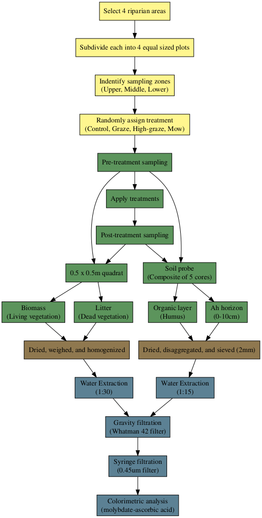
A randomized complete block experimental design was used to assess the sources of riparian WEP and investigate how it changes following cattle grazing or mowing treatments. In addition to a control, the three treatments included grazing, high-density grazing, and mowing. Each treatment, including a control, was replicated in riparian areas surrounding four prairie potholes (wetlands). Samples of biomass, litter, organic layer, and Ah horizon, were collected in three locations both pre- and post-treatment. A workflow diagram showing the experimental setup, field work, sample preparation, and laboratory analysis can be found in Figure S1.
The study was conducted at the Manitoba Beef and Forage Initiatives (MBFI) research farm (50.06\(^\circ\)N, 99.92\(^\circ\)W; 502 AMSL), approximately 25 km north of Brandon, Manitoba, Canada, in the Prairie Pothole region of North America (Figure 1). The normal (1981-2010) average daily air temperature was 2.2 \(^\circ\)C, and the cumulative annual precipitation at Brandon was 474.2 mm, with 24.8 % falling as snow (Environment and Climate Change Canada, 2024). The Köppen-Geiger climate classification is cold, without dry season, and with warm summer (Dfb) (Beck et al., 2018). The region is predominantly agricultural land use, including annual crops (grains and oil seeds) and grazing/forage. MBFI is a 260-hectare (ha) research and demonstration farm with a mix of pasture, hay, and forage/silage cropland. Prior to the establishment of MBFI the site was part of the Manitoba Zero Tillage Research Association farm (1993-2014) where annual crops, including oil seeds and grains, were grown.
There are also numerous small permanent and ephemeral wetlands (potholes) and associated riparian areas which account for approximately 35% of the total farmland (Manitoba Beef & Forage Initiatives, 2024). The riparian areas surrounding the larger permanent wetlands are fenced off to exclude livestock and are not actively managed. Approximately half the farm has an irregular undulating to hummocky relief (2-5%) with the reminder being nearly level (0-2%). The soils have developed on fine loamy, moderately calcareous glacial till. The drainage class in upper slope positions are well to rapidly draining while lower slope and riparian soils are poorly drained and primarily consist of Humic and Luvic Gleysols (Podolsky and Schindler, 1993). The surface texture class of the riparian soil is a clay loam and pH values range from 7.1 to 8.3 with a mean of 7.6. Generally the surface soil profiles surrounding theses prairie potholes can be described by a 1-10 cm organic layer overlying a 10-18 cm Ah horizon (Podolsky and Schindler, 1993). In the riparian areas used as part of this study the average depth of the organic layer was found to be approximately 1 cm for the upper and middle sampling locations and 2 cm for the lower sampling location. The Ah horizon was more than 10 cm deep at all sampling locations.
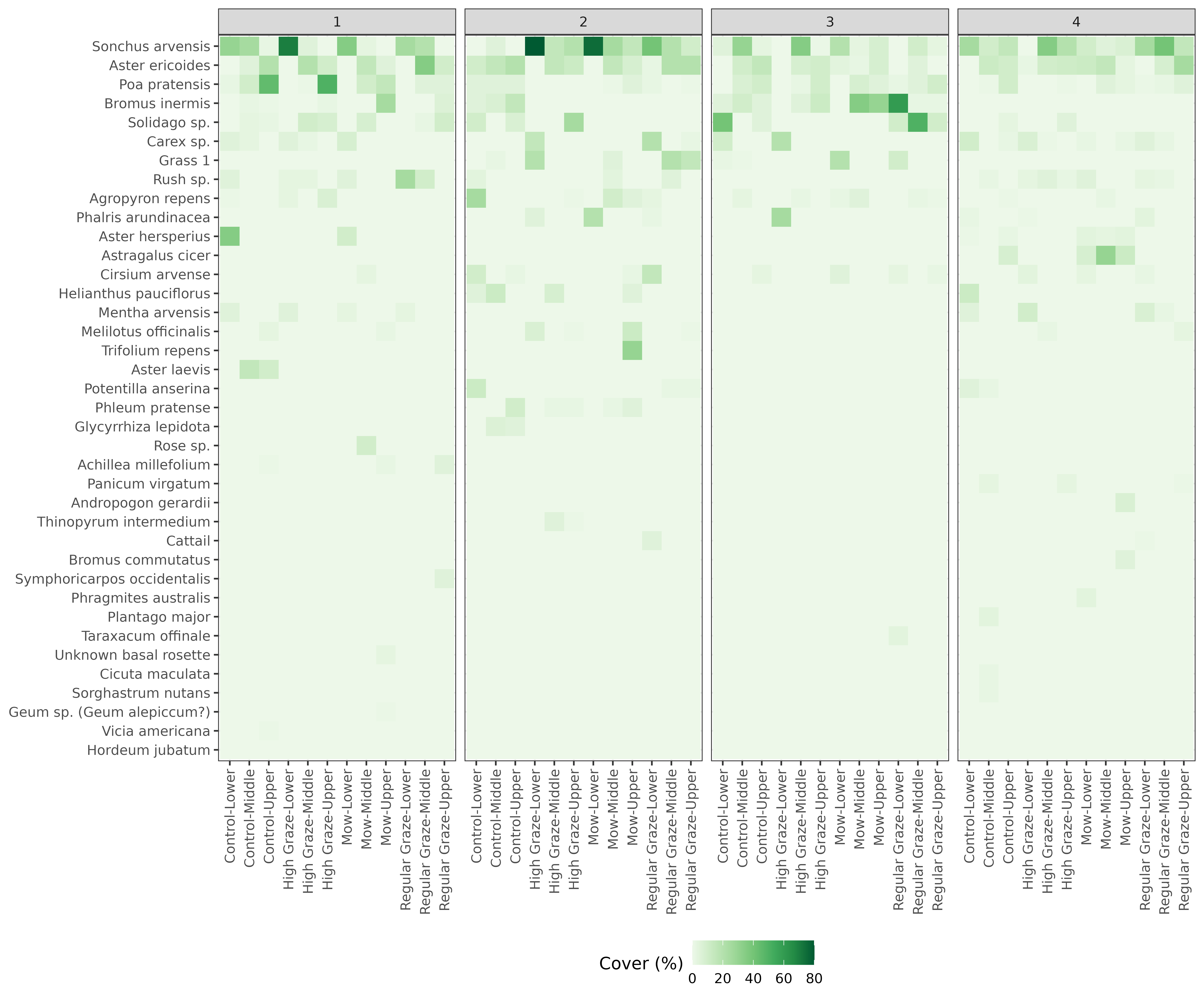
Vegetation was assessed using the foliar cover method for each plot within each of the four riparian areas. There was considerable variability among riparian areas, plots, and sampling locations (upper, midle, and lower). The four most dominant species identified were Sow Thistle (Sonchus arvensis), Smooth Aster (Aster laevis), Kentucky bluegrass (Poa pratensis), and Smooth Brome (Bromus inermis) and the complete assessment can be found in Figure S2. All riparian areas investigated in this study were adjacent to actively grazed pastures.
In [1]:
p6 <- p4 + inset_element(p1, left = 0.6, bottom = 0.6, right = 1, top = 1) + p5
p6Warning in st_point_on_surface.sfc(sf::st_zm(x)): st_point_on_surface may not
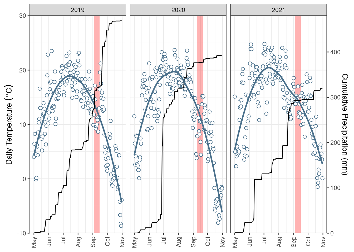
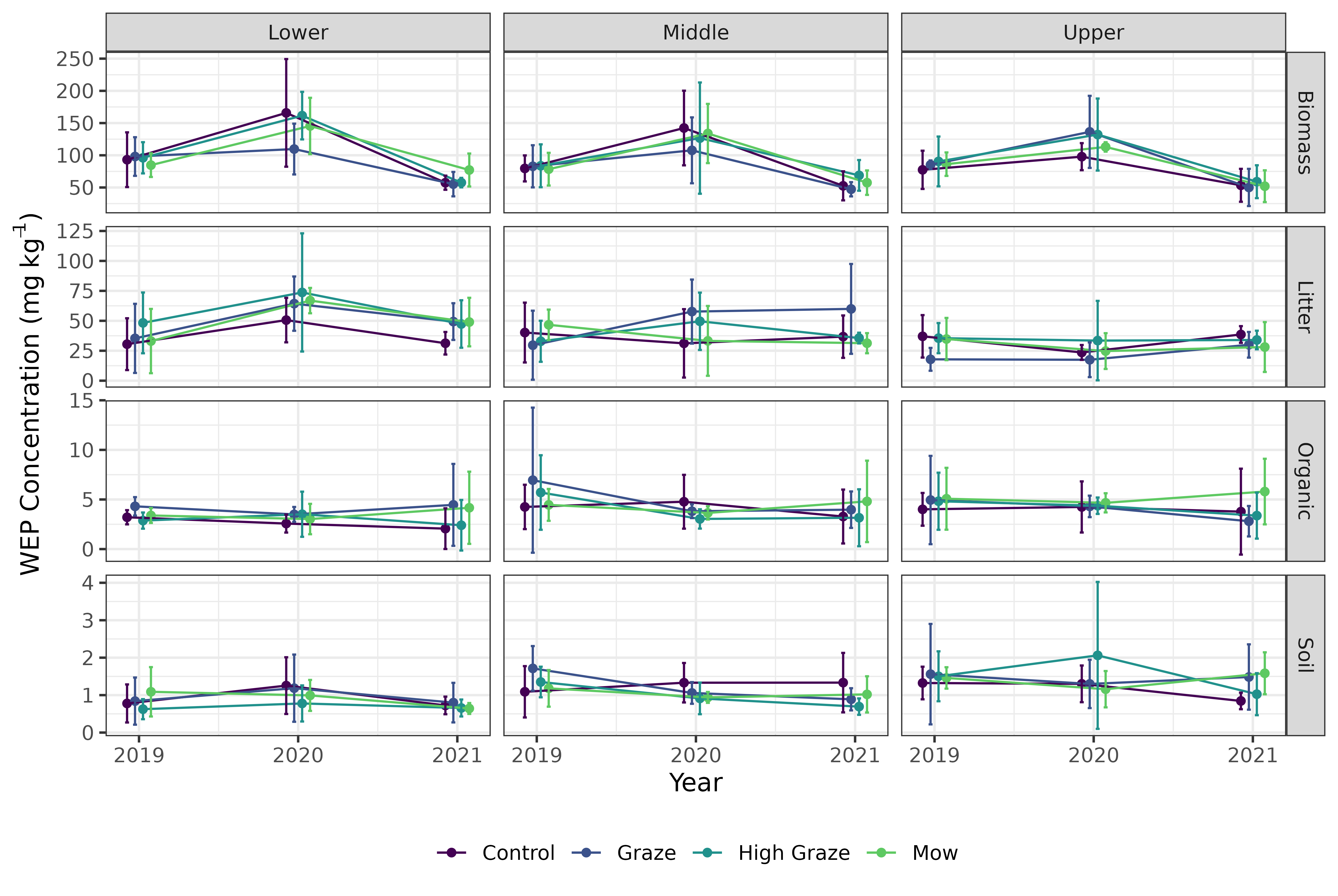
give correct results for longitude/latitude dataFour riparian areas surrounding permanent wetlands were selected (Figure 1) and subdivided into four approximately 450 \(m^2\) plots. Within each riparian area, each plot was randomly assigned to a treatment or control. The experimental groups (i.e., treatments) were 1) control, 2) graze, 3) high-density graze, and 4) mow and harvest. The grazing treatments consisted of a single five-hour grazing period, with the grazing treatment having 3.1-3.5 animal units per plot and the high-density grazing having 11.75-12 animal units. These stocking densities were used to approximate a typical rotational grazing and a mob grazing approach. The grazed plots were fenced on all four sides, including the edge of the waterbody and provided with supplemental water. The cattle grazing treatments occurred over four consecutive days where each day the graze and high-density graze treatments were completed at a given riparian area. The cattle were transported between the riparian areas by trailer and were placed in a holding area while not grazing the experimental plots. For the mowing treatment, the vegetation was cut to a height of 10cm, and the vegetation was manually raked out of the plot. Treatments were applied early to mid-September, before the first frost, in three consecutive years (2019-2021) (Figure S3). Within each plot three distinctive sampling locations, or topographic positions, were established, adjacent to the edge of the waterbody (lower), adjacent to the field/pasture (upper), and at the mid-point (middle). Samples were collected at each sampling location 1-3 days before and 1-3 days after treatment (including the control) to assess the impact of grazing and mowing. Before and after samples were collected at immediately adjacent locations.
Four types of samples were collected: 1) biomass, 2) litter, 3) organic layer, and 4) Ah horizon. Using a 0.25 \(m^2\) quadrate, biomass was collected by cutting the standing live vegetation and litter by raking the surface and picking up the previous year’s growth. Both the biomass and litter were dried at 40 \(^\circ C\), weighed, and homogenized using a blade grinder (<1cm). A composite of five soil samples was collected within the same quadrat as the biomass/litter using a 19 mm diameter soil probe and was divided into the organic layer (1 – 2 cm deep) and the top 10 cm of the Ah horizon. The organic layer and Ah soil were air-dried, disaggregated with a mortar and pestle, and passed through a 2-mm sieve. Additional bulk density samples of both the organic layer and Ah and the depth of the organic layer were collected in 2023. Daily air temperature and rainfall data were collected from an onsite station (Figure S3) (Manitoba Agriculture, 2023).
Water Extractable Phosphorus (WEP), an environmental soil and vegetation P test, was used to infer soil P release into runoff water. Dried and homogenized samples were extracted by shaking (150 RPM) with deionized water for one hour at a mass-to-volume ratio of 1:30 for the biomass and litter samples (1 g) and 1:15 for the organic and Ah samples (2 g). Extractions were gravity filtered through a Whatman 42 filter followed by syringe filtration with a 0.45 \(\mu m\) nylon filter. WEP in the extract was measured spectrophotometrically by the colorimetric molybdate–ascorbic acid method (Murphy and Riley, 1962; Sharpley et al., 2006).
The concentration of WEP (\(mg~kg^{-1}\)) was calculated for all sources of P. In addition, the areal density of WEP was calculated for biomass and litter by combining WEP concentration with the mass of material collected from the quadrat. The vertical profile of WEP within the riparian area assessed from samples collected before treatments were implemented across the 3-year study. For comparison, an approximate estimation of areal density WEP in the organic layer and Ah was calculated using the bulk density and depth measurements collected in 2023 (Figure 2 b).
All statistical analysis, plotting, and mapping were undertaken using the R Statistical Software (v4.4.3; R Core Team (2024)), through the RStudio Integrated Development Environment v2023.12.1.402 (RStudio, 2024). All plots and maps were created using the R package ggplot2 (v3.5.1; Wickham (2016)). Country and regional maps were created using data from the rnaturalearth package (Massicotte and South, 2023) and other maps using ESRI imagery and the OpenStreetMap package (Fellows, 2023). Four Linear Mixed Models (R package glmmTMB v1.1.10; Brooks et al. (2017)) were used to investigate the effect of treatment and riparian sampling location (including interaction) on the numeric difference in WEP measurements taken before and after treatment for each of the four distinct sources of P (areal densities for biomass and litter; concentrations for organic matter and Ah). Year and riparian area were included as crossed random factors to control for the variability within years and riparian areas.
Additionally, when investigating the net change in biomass WEP the initial biomass WEP (before applying the treatment) was included in the model as a covariate. This controls for the fact that the magnitude of the difference in biomass measurements taken before and after treatment is directly related to the mass of WEP initially available. By controlling for this, the model indicates which treatments resulted in a relatively greater change in biomass, rather than simply absolute change.
The interaction between treatment and riparian sampling location was removed if non-significant (p < 0.05). When a main effect or interaction was significant, post-hoc pairwise comparisons with a Benjamini-Hochberg p-value adjustment were performed (p <0.05). When a main effect or interaction was significant, post-hoc pairwise comparisons with a Benjamini-Hochberg p-value adjustment was used (emmeans v1.10.6; Lenth (2024)). Model assumptions were assessed using DHARMa residual plots (DHARMa v0.4.7; Hartig (2022)), main effects were tested for collinearity (performance v0.12.4; Lüdecke et al. (2021)), and results were presented as type III ANOVA (car v3.1.3; Fox and Weisberg (2019)). For each unique source of WEP, the null hypotheses were 1) no difference in the net WEP among treatments or riparian sampling locations and 2) no interactions between these two factors.
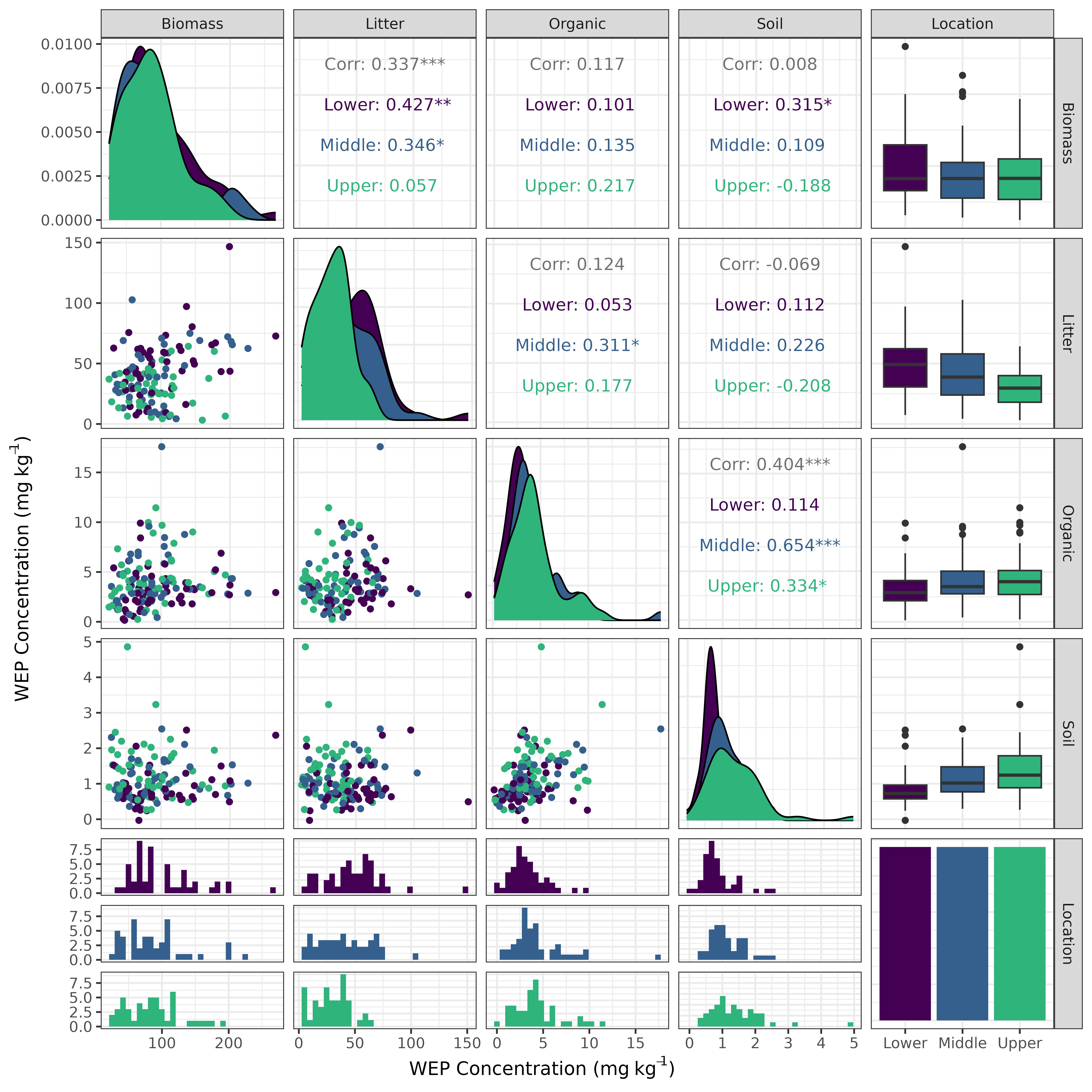
Pearson correlations were performed to explore relations in WEP concentrations among the four unique P sources for each of the three topographic positions using samples collected before the application of the treatments. These relations were visualized using a scatterplot matrix created using the GGally R package (v2.2.1; Schloerke et al. (2024) )
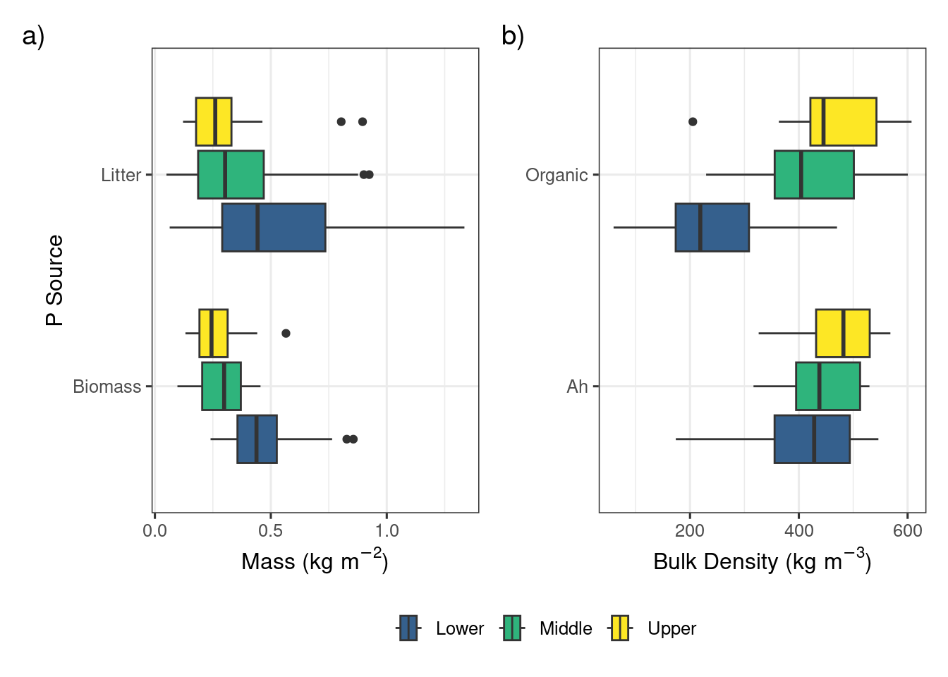
The biomass, litter, organic layer, and Ah horizon sources of P demonstrated a strong vertical stratification in both the concentration and areal densities of WEP (Figure 2). The median concentrations in the vegetation sources were 82.8 and 39.0 \(mg~kg^{-1}\) for the biomass and litter components, respectively, which is more than an order of magnitude greater than the soil components (0.9 and 3.4 \(mg~kg^{-1}\); Ah and organic, respectively). Considerable variability in the WEP concentration in the biomass and litter sources were observed with interquartile ranges (IQR) of 54.3 and 32.9 \(mg~kg^{-1}\) for the biomass and litter sources, respectively. In contrast, the IQR for the organic and Ah sources both were <2.5 \(mg~kg^{-1}\).
Overall, in terms of the areal density of WEP, the top 10 cm of the Ah horizon was the largest source of WEP (42.5 \(mg~m^{-2}\)) followed by the biomass (26.3 \(mg~m^{-2}\)), organic layer (14.3 \(mg~m^{-2}\)), and the litter (13.7 \(mg~m^{-2}\)). It should be noted that these are only approximate estimates for the organic layer and Ah horizon because the values for depth and bulk density measured in 2023 were used in the calculations for all previous years (Figure S4). Nevertheless, the vertical profile of WEP in riparian areas (Figure 2) observed in this study supports the concept that a measure of P in soil alone is likely missing a large proportion of the near-surface P that can be potentially lost during the spring snowmelt (Liu et al., 2019a; b; Cober et al., 2019). The substantial proportion of WEP above the soil surface provides evidence that managing the biomass in riparian areas in autumn may reduce the contribution of P lost directly from this area during spring. Specifically, the harvesting of this biomass results in an export of P which can maintain or enhance the buffering or storage capacity of P derived from upslope sources further improving downstream water quality (Kelly et al., 2007; Hille et al., 2019).
In [2]:
p3 <- p1+p2 + plot_layout(guides = 'collect') & theme(legend.position = 'bottom', legend.title = element_blank())

p3
Warning: Removed 2 rows containing non-finite outside the scale range
(`stat_boxplot()`).
Removed 2 rows containing non-finite outside the scale range
(`stat_boxplot()`).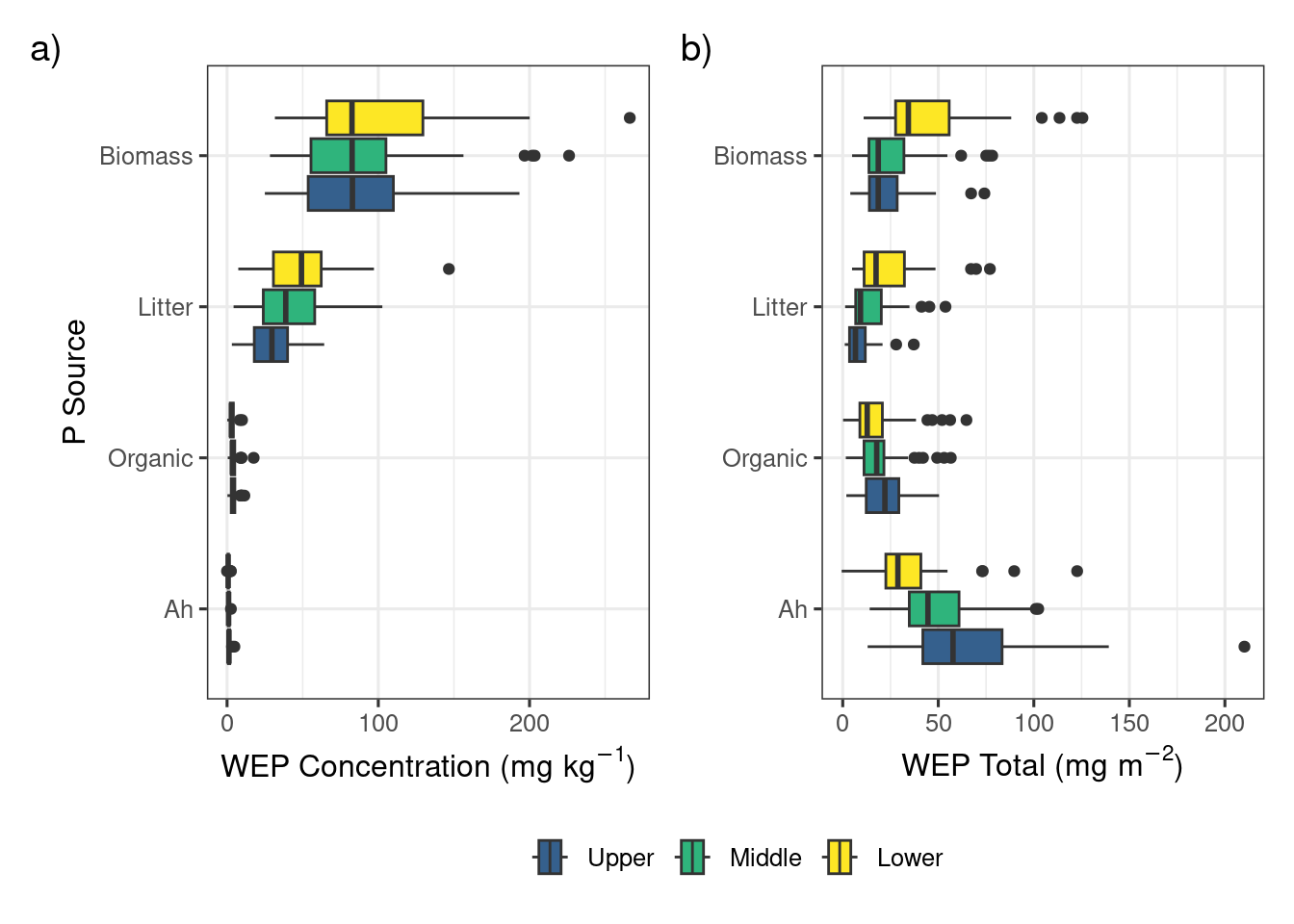
Prior to grazing and mowing treatments, the median WEP concentrations were similar among the upper, mid, and lower positions for the biomass samples. There was a small topographic trend in the WEP concentration for both the Ah and organic litter P sources where the concentration decreased from the upper through to the lower sampling locations. The WEP concentrations in the Ah and organic layer were found to be significantly (p < 0.001) and positively correlated (r2 = 0.40) (Figure 2 and Figure S5). This topographic pattern is consistent with other studies and is likely due to the rapid physical and geochemical retention of upslope derived P within the first 5 m of the riparian area (Syversen and Borch, 2005).The litter showed the opposite topographic trend with higher WEP concentrations in the lower sampling locations. There was a significant (p < 0.001) positive correlation (r2 = 0.34)between the WEP concentration in the biomass and litter samples suggesting that biomass with a high WEP concentration produces litter with a high WEP concentration (Figure S5). There was no correlation (p > 0.05) between the Ah and biomass WEP concentrations suggesting that higher soil WEP concentration does not result in biomass with elevated WEP concentrations at this study site (Figure S5). There is some evidence that plants growing in P-rich environments can become enriched in P (e.g., Kröger et al., 2007); however, there was no correlation (p > 0.05) between the Ah and biomass WEP concentrations suggesting that higher soil WEP concentration does not result in biomass with elevated WEP concentrations at this study site (Figure S5).
For the biomass and litter sources, the lower riparian locations had greater areal densities of WEP whereas the organic and Ah sources had greater areal densities of WEP in the upper riparian locations. The longitudinal gradient of WEP showed an inverted symmetry where the biomass WEP was largest near the lower sampling location and the Ah soil WEP was largest in the upper sampling location adjacent to the fields (Figure 2 b). The high soil water content in the lower location created conditions that favor high biomass production (Figure S4) and higher WEP concentration (Figure 2 a). The higher bulk density was most likely due to the lower soil organic matter content and the higher WEP concentration may be related to the interception of P-rich runoff from upslope areas (Tomer et al., 2007). Understanding and quantifying the sources and patterns of P within riparian areas is a key part of assessing the risk of P loss as it helps to inform management decisions and target the largest sources of P (Reid et al., 2018).
There was considerable variation across all treatments and riparian locations in all four P sources. This high variability in WEP areal density/concentration is best reflected in the control treatment where the expected difference was 0 (Figures 3 through 6), but WEP losses and gains were still observed despite no treatment being applied. . For example, the control plots had a median biomass WEP removal rate of 5.5 \(mg~m^{-2}\) (Figure 3 a). However, despite this variability, several patterns demonstrating relationships among treatments and vertical and longitudinal P emerged.
Results of the linear mixed model of areal density of biomass WEP show a significant effect of treatment (X2 = 24.8, df = 3, p < 0.001) and riparian location (X2 = 15.7, df = 2, p < 0.001). Post-hoc comparisons showed that the net biomass WEP for the high-density grazing and mowing treatments were similar (p>0.05) but significantly (p<0.05) different from the control and graze treatments (Figure 3 a and Table 1).The mowing and high-density grazing reduced the average WEP areal density by 7.4 and 4.2 \(mg~m^{-2}\) relative to the control, respectively. The reduction in biomass WEP was significantly (p<0.05) greater in the lower sampling locations as compared to the upper and mid locations (Figure 3 b and Table 1) with a difference in average WEP of 10.2 \(mg~m^{-2}\) between the lower and upper locations of the riparian area.
In [3]:
p3 <- p1 + p2 + plot_layout(guides = 'collect') & theme(legend.position = 'bottom', legend.title = element_blank())
p3
Warning: Removed 2 rows containing non-finite outside the scale range
(`stat_boxplot()`).
Removed 2 rows containing non-finite outside the scale range
(`stat_boxplot()`).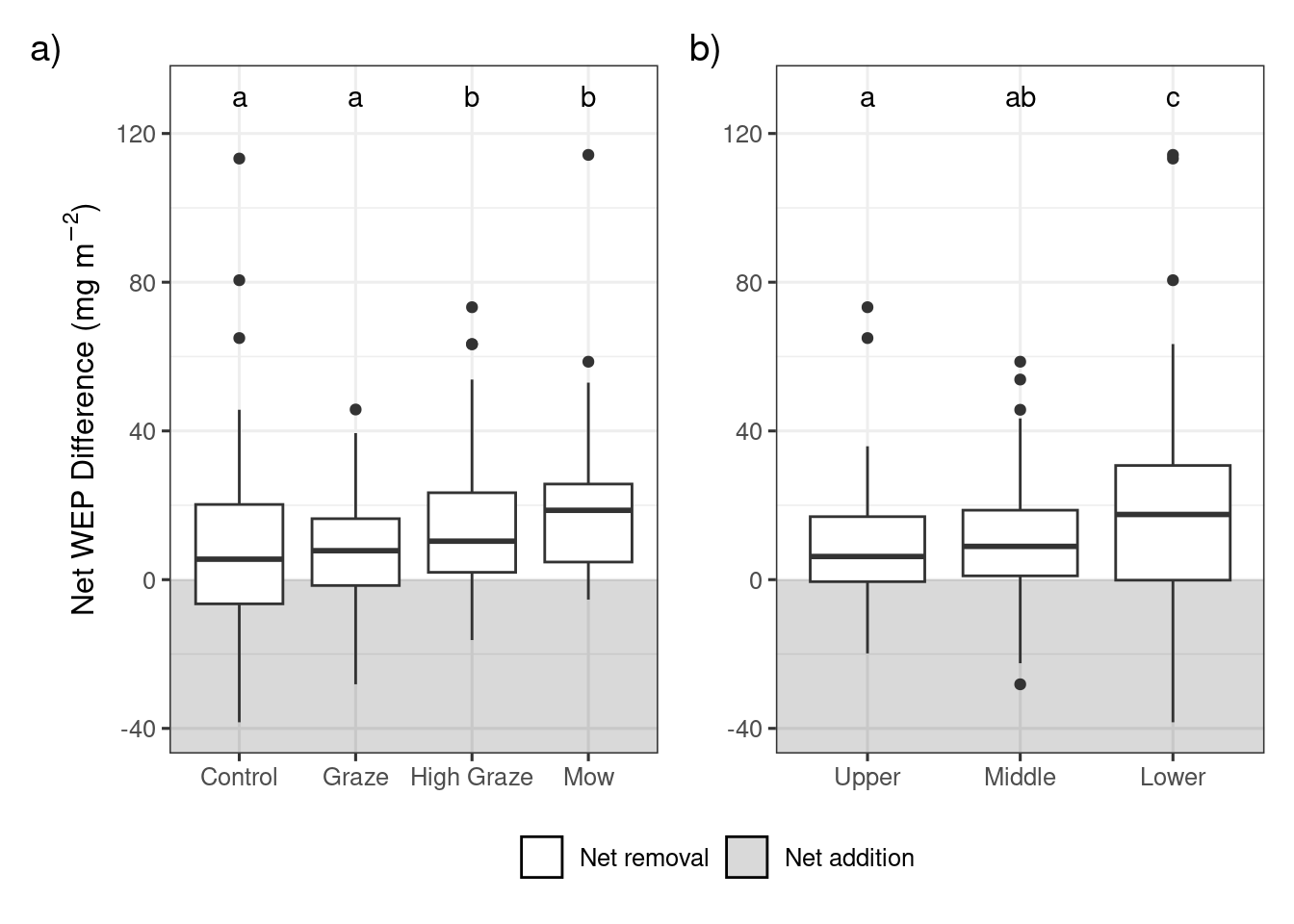
The model looking at areal density of litter WEP showed no significant impacts of either treatment (X2 = 1.15, df = 3, p = 0.23) or riparian location (X2 = 4.30, df = 2, p = 0.56) (Figure 4). ). In contrast, the model exploring WEP concentration in the organic layer (Figure 5) detected no significant difference among riparian locations (X2 = 0.57, df = 2, p = 0.75) but did find a significant effect of treatment (X2 = 8.24, df = 3, p = 0.04). However, the post-hoc pairwise comparisons (Table 2) found no significant differences (p < 0.05) among the treatments. Finally, there was no significant effect of treatment (X2 = 2.59, df = 3, p = 0.46) or riparian position (X2 = 1.17, df = 2, p = 0.56) on the concentration of WEP in the Ah horizon (Figure 6).
In [6]:
p1 <- ggplot(data = filter(plot_data, measure == "p_total")) +
  theme_bw(base_size = 12) +
  geom_rect(data = df, aes(xmin = x1, xmax = x2, ymin = y1, ymax = y2, fill = difference), alpha = 0.15) +
  #scale_fill_manual(values = c("white", "black")) +
  #ggnewscale::new_scale_fill() +
  geom_boxplot(aes(x = treatment, y = diff, fill = location)) +
  labs(y = expression(paste("Net WEP Difference (", mg~m^{-2}, ")")), x = "Treatment") +
  #scale_fill_viridis_d(name = "Location", begin = 0.3, end = 1) +
  scale_fill_manual(values = c("white", "black", "#35608DFF", "#2FB47CFF", "#FDE725FF")) +
  guides(fill = guide_legend(override.aes = list(colour = "black", size = 1))) +
  theme(axis.title.x = element_blank(),
        axis.text.x = element_text(angle = 0, vjust = 1, hjust = 0.5),
        legend.position = "bottom",
        legend.title = element_blank())
p1
Warning: Removed 11 rows containing non-finite outside the scale range
(`stat_boxplot()`).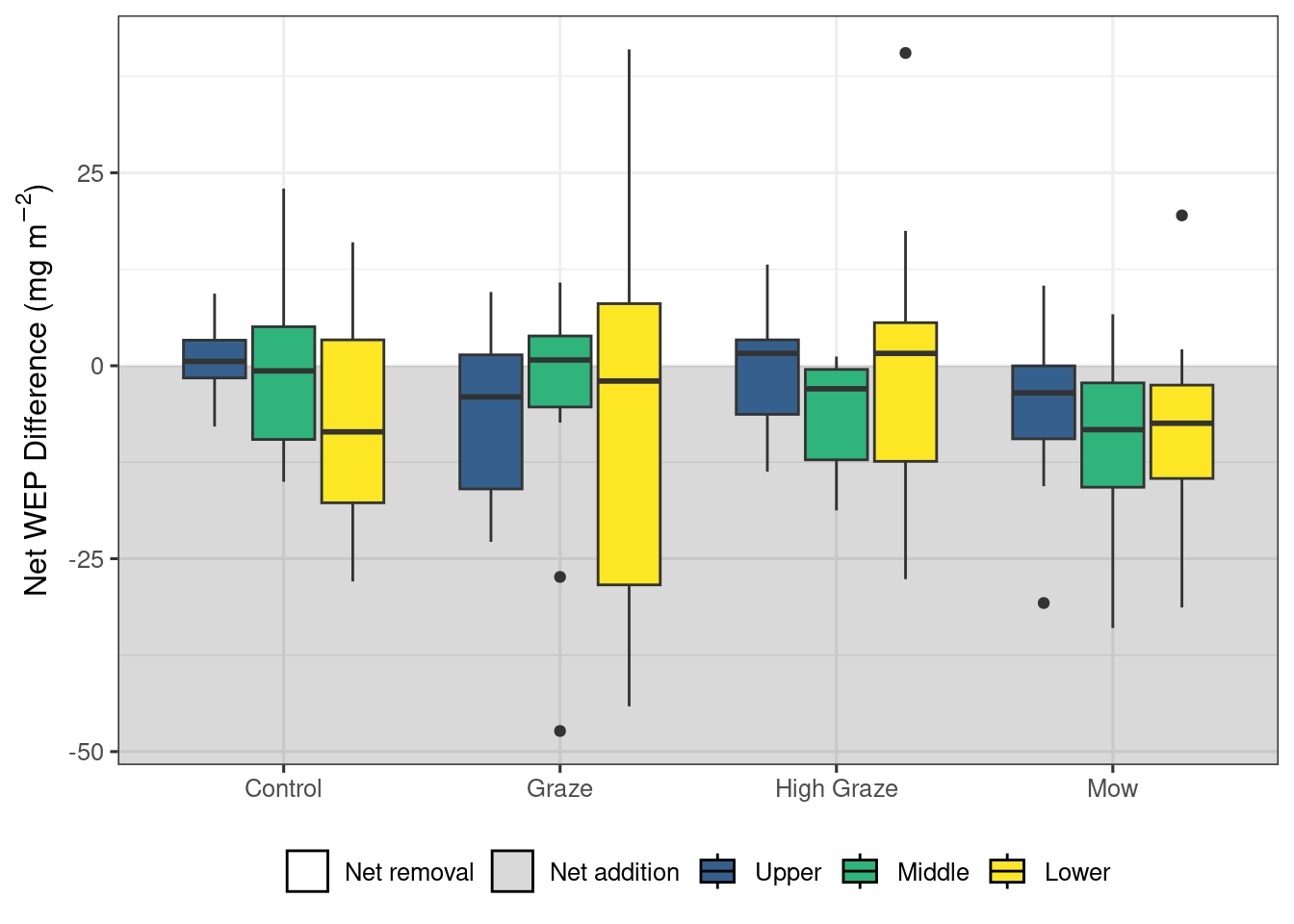
In [7]:
p1 <- ggplot(data = organic_diff) +
  theme_bw(base_size = 12) +
  geom_rect(data = df, aes(xmin = x1, xmax = x2, ymin = y1, ymax = y2, fill = difference), alpha = 0.15) +
  #scale_fill_manual(values = c("white", "black")) +
  #ggnewscale::new_scale_fill() +
  geom_boxplot(aes(x = treatment, y = diff, fill = location)) +
  #scale_fill_viridis_d(name = "Location", begin = 0.3, end = 1) +
  scale_fill_manual(values = c("white", "black", "#35608DFF", "#2FB47CFF", "#FDE725FF")) +
  guides(fill = guide_legend(override.aes = list(colour = "black", size = 1))) +
  labs(y = expression(paste("Net WEP Difference (", mg~kg^{-1}, ")")), x = "Treatment") +
  theme(axis.title.x = element_blank(),
        axis.text.x = element_text(angle = 0, vjust = 1, hjust = 0.5),
        legend.position = 'bottom', legend.title = element_blank())
p1
# ggsave(plot = p1, filename = here::here("./Figures/Figure 5.tiff"), width = 174, height = 85, units = "mm", dpi = 400)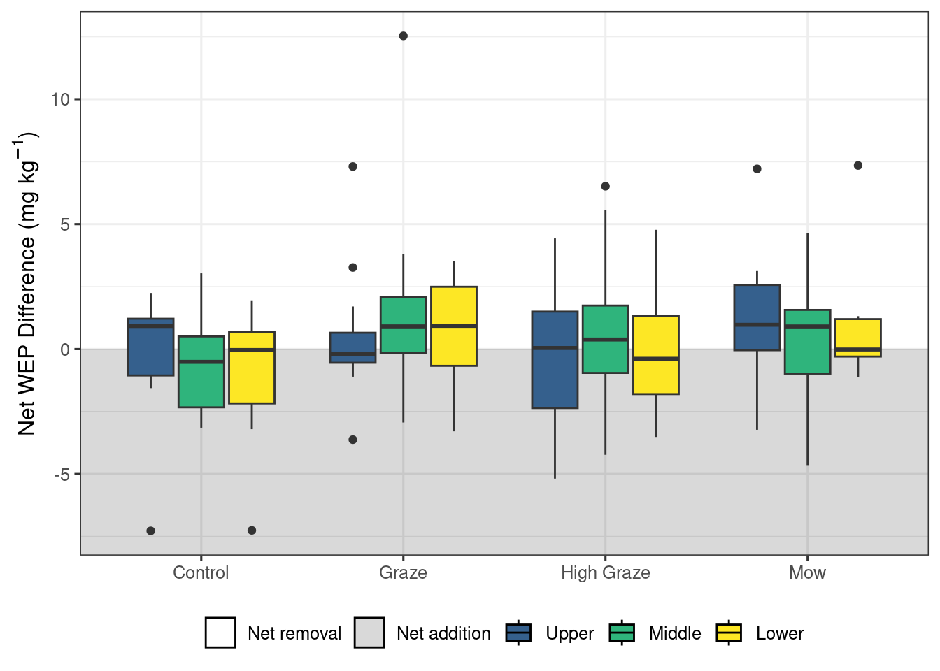
In [10]:
p2 <- ggplot(data = soil_diff) +
  theme_bw(base_size = 12) +
  geom_rect(data = df, aes(xmin = x1, xmax = x2, ymin = y1, ymax = y2, fill = difference), alpha = 0.15) +
  #scale_fill_manual(values = c("white", "black")) +
  #ggnewscale::new_scale_fill() +
  geom_boxplot(aes(x = treatment, y = diff, fill = location)) +
  #scale_fill_viridis_d(name = "Location", begin = 0.3, end = 1) +
  scale_fill_manual(values = c("white", "black", "#35608DFF", "#2FB47CFF", "#FDE725FF")) +
  guides(fill = guide_legend(override.aes = list(colour = "black", size = 1))) +
  labs(y = expression(paste("Net WEP Difference (", mg~kg^{-1}, ")")), x = "Treatment") +
  theme(axis.title.x = element_blank(),
        axis.text.x = element_text(angle = 0, vjust = 1, hjust = 0.5),
        legend.position = 'bottom', legend.title = element_blank())
p2
# ggsave(plot = p2, filename = here::here("./Figures/Figure 6.tiff"), width = 174, height = 85, units = "mm", dpi = 400)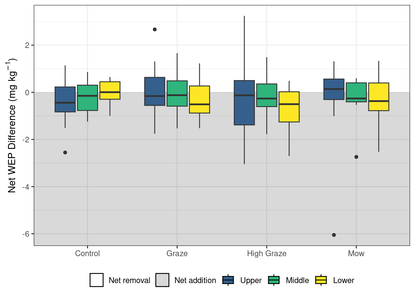
Taken together, these results suggest that short-term autumn high-density grazing may be a potential management tool that can reduce the mass of P lost directly from the riparian area (Figure 3 a). In addition to managing P loss, grazing riparian areas can also provide an essential source of forage, particularly during drought. Mechanized harvesting of biomass could also achieve this reduction in P loss (Figure 3 a) if the landscape and soil conditions are favorable. Despite the cycling of nutrients by the removal of P through grazing of biomass (Figure 3) and the deposition through excretion, no differences were detected in the litter and Ah sources of P (Figure 4, and 6). The models did detect a significant effect of treatment on the organic layer WEP; however, the pairwise comparisons were not able to detect any significant differences and the exact nature of the impact of the treatments remains unclear.
The ability to detect changes in the WEP sources in riparian areas is difficult due to spatial variability in both the pre- and post-grazing treatments. Even within the control plots, both net addition and removal of WEP were detected and in many cases the variability was similar to the other treatments. This inherent variability (i.e., pre-grazing) likely results from a combination of hydrological factors like ground water fluctuations, soil attributes such as texture, ecological dynamics involving plant community composition, and anthropogenic influences like historical land management practices (McClain et al., 2003; Vidon et al., 2010). In particular, the species cover information (Figure S2) demonstrates a wide range in species composition and abundance, this coupled with the variation in P release with different vegetation species may explain some of the observed variability (Cober et al., 2018).
The prairie pothole wetlands regularly experience high water levels in the early spring. Automated observations made with a water level logger adjacent to one plot between October 2020 and May 2021 showed that the lower, middle, and upper sampling points experienced inundation for approximately 21, 11, and zero days, respectively (Noyes et al., 2024). The annual weather conditions and topography of riparian areas surrounding the wetlands will impact the length and extent of flooding. Prolonged contact with water has been shown to increase the mass of WEP lost in both soil (Young and Briggs, 2008) and vegetation (Lozier and Macrae, 2017) and may also explain some of the observed variability. As reported by Podolsky and Schindler (1993), the soils surrounding these potholes are typically low in CaCo3 and have a neutral to slight alkaline pH. In this pH range (6.5 to 7.5) P availability is typically at its highest and not expected to precipitate with Ca. A more detailed soil chemical analysis, particularly Fe and Mn, along with soil saturation duration information (i.e., redox) would be needed to fully assess the potential for P loss during the spring (Walton et al., 2020).
The WEP protocol used for both soil and vegetation samples are not likely to capture redox-sensitive mobilized P from the soil (Walton et al., 2020) or enhanced P leaching from vegetation (Lozier and Macrae, 2017). Similarly, the WEP protocol also does not capture the enhanced P release from soil and vegetation that results repeated freeze-thaw cycles (Liu et al., 2013; Lozier and Macrae, 2017). However, temperature sensors placed at the soil surface adjacent to one plot recorded four freeze-thaw cycles between Oct 2020 and May 2021 and found that surface temperatures fluctuations are moderated in this region by the relatively persistent snowpack (Noyes et al., 2024).), reducing the potential effects of freeze-thaw cycles on P release. However, both the prolonged contact with water and freeze-thaw cycles are not captured in the WEP protocols and may result in an underestimation of the potential for P loss from each of the four distinctive sources of P in riparian areas.
In addition to climatic effects, there may be variability in P as a side effect of the study design. One source of variability could be from added urine and manure in grazed areas which likely created additional hotspots of P that may carry forward to subsequent years (Subedi et al., 2020; Donohoe et al., 2021). However, there was no indication of P accumulation due to grazing in any of the four distinctive P sources over the 3-year study period. The highest concentrations of WEP were typically found in the second year of the study (Figure S6). This suggests that other biophysical processes regulated by weather conditions (Figure S3) were of greater importance in controlling the WEP concentrations than P additions from cattle urine and manure.
Another source of variability may have been from sampling. As there was significant variability among plots, the single 0.25 \(m^2\) sampling quadrat within each riparian location may have been insufficient to capture the spatial variability. Therefore, larger composite and/or several sampling locations within each upper, middle and lower locations are recommended. Appropriate sampling design becomes critical as the scale of observation of similar research increases to the farm scale, and so will the range and sources of variability. As the scope of research is expanded to the farm level, the importance of using an appropriate sampling design becomes increasingly critical (Hale et al., 2014).
Autumn was selected for the mowing and grazing treatments for three reasons. The first was to reduce the mass of biomass P available that can contribute to the P loss during the spring snowmelt. Second, drier soil conditions reduce the extent of pugging and soil compaction, which limits the disruption of soil structure and damage to plants (Batey, 2009). Lastly, the prairie potholes and associated riparian areas are important breeding habitats for migratory birds. Grazing can negatively affect these species, but late-season grazing may reduce this potential ecological impact (Stanley and Knopf, 2002). However, the type of grazing system (timing, stocking rate, and density, etc.) may impact habitat quality and breeding success (Carnochan et al., 2018; Hansen et al., 2019; Kraft et al., 2021).
Corridor fencing at the edge of the waterbody and alternative water sources were used in this study to limit livestock access to prevent bank erosion and protect water quality (e.g., direct deposition) (Dauwalter et al., 2018). Scaling this to the farm level would require virtual fencing or infrastructure (Aarons et al., 2013) and time (to conduct short-term grazing), especially in prairie pothole region where there are numerous and small riparian areas (Sovell et al., 2000; Hubbard et al., 2004; Hulvey et al., 2021; Manitoba Agriculture, 2024).
The long-term impacts of repeated grazing of riparian areas also need to be considered. From a nutrient loss reduction perspective, a shift in the magnitude of P sources could be expected as less biomass is available to be added to the litter source, affecting the organic layer and Ah sources of P. The regular inclusion of cattle will also introduce a new manure source of P, which can spatially redistribute P and initially be more water soluble and readily transported (Franzluebbers et al., 2019). Grazing can also reduce the litter layer through trampling increasing the soil-vegetation contact and speeding up the decomposition process. These changes in biomass and litter quantities may result in changes to habitat structure. Although this study generally considers environmental implications, forage management practices also have an agronomic effect which should be taken into consideration when developing best management practices (Subedi et al., 2020).
Biomass and litter are significant sources of near-surface WEP in riparian areas that have been historically disregarded in studies. Management of the biomass prior to the onset of winter conditions in cold climates has the potential to reduce the mass of P directly lost during the spring snowmelt and maintain or enhance the nutrient buffering capacity. The results from this experiment demonstrated that short-term, high-density cattle grazing and mowing both resulted in a reduction in the mass of biomass WEP, particularly in the lower riparian locations. The grazing and mowing treatments had no detectable effect on the other three near-surface sources of WEP. However, detecting changes in the near-surface sources of WEP is challenging due to high spatial variability.
Additional work on riparian management strategies is needed to address the specific challenges posed by cold climates. In these regions, the runoff and nutrient losses occur predominately during the spring snowmelt period when the ability of riparian areas to trap and retain nutrients is diminished. Further, the repeated freeze-thaw cycles of the vegetation and soils increases the potential P losses during this key time. Continued research to identify, quantify, and manage these sources of P to improve water quality remains a priority. In addition to improving water quality, the development of riparian management strategies should prioritize the protection of other ecological goods and services and recognize these areas as an integral part of the farm.
This project was undertaken with the financial support of the Government of Canada through the federal Department of Environment and Climate Change and a Lake Winnipeg Basin Program grant awarded to the Manitoba Association of Watersheds. Additional research funding was provided through a Brandon University Research Committee grant awarded to AK. Thank you to A. Avila, M. Luna, C Sobchuk, and A. Tan for all the help with lab and field work. Special thanks to the Manitoba Beef and Forage Initiatives research farm staff for the use of their facilities and managing the cattle grazing and mowing treatments. Lastly, thank you to R. Canart and M. Elsinger for helping to develop the experimental design.
Data and source code for analysis and manuscript available on GitHub: https://github.com/alex-koiter/riparian-grazing-manuscript
Data set also available in the Dryad repository: https://doi.org/10.5061/dryad.nzs7h4526
The authors have no competing interests to declare that are relevant to the content of this article.